Published January 2026 - Based on EVS Version 2026.1.0

Please see the video below for details on updates to the user interface in EVS 2026.1. Alternatively, view this on Guidde directly.

00:00: Earth Volumetric Studio 2026.1 introduces a streamlined user interface designed to boost your productivity and simplify workflows. This update focuses on reducing clutter and optimizing usability for all users.

00:16: Version 2026.1 contains a major user interface update focused on simplification across the board.

00:24: The user interface has reorganized to focus on key functionality, enhancing productivity and optimizing screen real estate on laptops and multiple monitors.

00:33: Let’s start with the changes beginning right at startup with a brand new startup screen. Notice the new, simpler screen.

00:40: Along the top are buttons to open an existing or create a new application.

00:47: You can also see your recent files, which now include preview screens so you can see what each application contained.

00:55: At the bottom of the window, there are links to recent tips and tricks to help you get the most out of the software.

01:02: Clicking any of these links will open the tips and tricks page in your web browser for easy access.

01:07: Let’s go ahead and open an application so we can explore the new interface in action.

01:12: The first key change is a brand new much simpler toolbar with detailed tool tips on all buttons.

01:20: There are far fewer options on the toolbar now, streamlining your workspace.

01:25: Most missing options have been moved to more logical places, such as application properties like Z Scale and Explode now accessible directly in the application window.

01:35: The toolbar supports different views to optimize screen space, from full size to compact, ideal for laptops or experienced users.

01:44: On the far right of the screen, a small menu provides access to all of the density options

01:50: The compact setting uses small icons with tooltips to maximize screen real estate while maintaining usability.

01:56: On laptops, or if you want to maximize screen real estate, you can even move the toolbar all the way up to the application title bar to provide the most screen space.

02:07: Here I choose the comfortable toolbar setting for a balanced mix of space and usability.

02:13: In previous versions, tools were in ribbon tabs; now all tools have been moved into detailed submenus for better organization.

02:21: Each tool now includes detailed tooltips to help you understand their functions and select the right one.

02:29: Options have been moved from the ribbon to a reorganized options screen.

02:35: The Options screen is now organized into two sections. User preferences on the left include options which affect the current user, such as switching between light and dark themes. The left panel options do not alter your data or applications.

02:49: The settings on the right side of the options window let you change defaults for instancing modules or creating new applications.

02:56: Close the options window to return to the main Application interface.

03:01: Now we will focus on improvements to the Application Window. The Application Window can now be dragged out and moved to a second monitor for improved multi-screen workflows.

03:11: Modules and the application overview are no longer their own Windows, and are now part of the main application window for better cohesion.

03:19: Modules are kept within the application window since they are only usable within your application context.

03:25: The modules window can be pinned or unpinned to auto-hide, which is useful on smaller screens or laptops.

03:31: Auto-hiding the modules pane helps maximize workspace on smaller screens or laptops.

03:37: Use the Modules Button in the Application toolbar, or press Control plus M to open the modules pane when needed.

03:43: A search bar at the top helps you quickly find modules by name or type within your application.

03:50: Typing keywords like ‘slice’ shows all modules matching that name or type for easy access.

03:57: Clicking a module centers it in your application and activates its properties for editing.

04:03: Select a module from the search results to work with its properties.

04:06: Notice that Slice Y is now centered in our Application, as well as having it’s properties selected for editing in the Properties Window.

04:14: Application wide options have been reworked significantly for this release.

04:19: What used to be called application properties is now renamed to application favorites.

04:26: Editing application favorites lets you manage properties from any modules you’ve marked as favorites.

04:33: You can add any property of a module, such as the current state of a sequence, to your application favorites for quick access.

04:40: Select a module to include its property in your application favorites.

04:45: Clicking to the left of a property adds it to the Application Favorites.

04:50: In this case, the current state will now appear in your application favorites.

04:55: The Application Favorites will also be available when creating an EVS Presentation Application.

05:02: A new application properties window contains application-wide settings like Z Scale and Explode.

05:09: Features previously in the ribbon, such as project and status information, are now included in the application properties window along with coloring options.

05:17: The application properties window also includes new features like Python assets and bookmarks.

05:23: Application favorites and application properties are separate, but switching between them is easy.

05:29: A button at the top will switch back and forth between Application Favorites and Application Properties

05:37: Thank you. If you have any questions, always feel free to contact support. And I hope you enjoy the new release.

05:44: Get started immediately by exploring the simplified interface and new features in Earth Volumetric Studio 2026.1. For additional help, visit our support resources or contact support anytime to ensure a smooth transition.

Published September 2025 - Based on EVS Version 2025.6.0

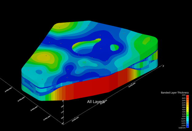
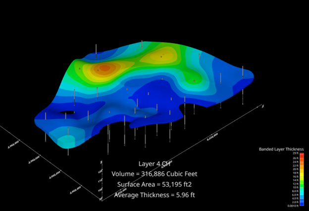
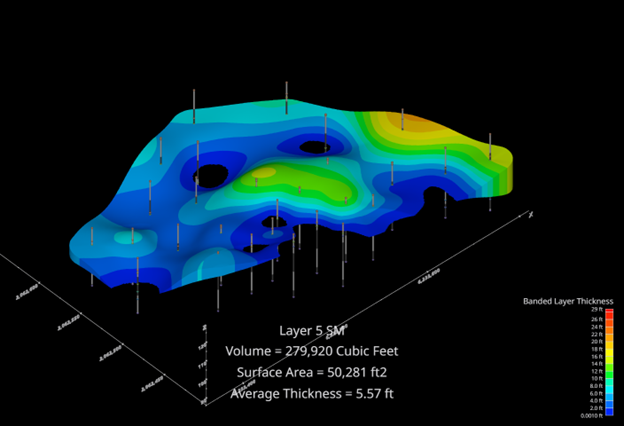
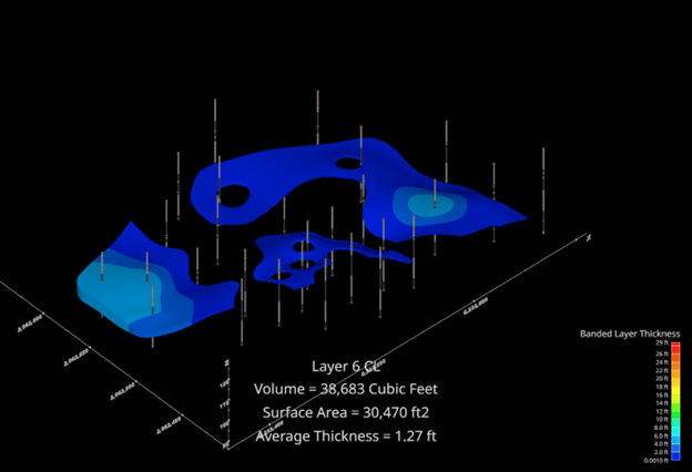
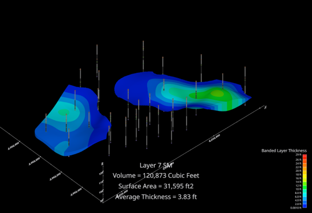
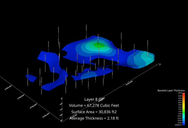
Calculating the average thickness of a geologic layer is straight forward if the layer is continuous across the model domain. The first step is to calculate the volume of the layer, then divide it by the surface area of the layer to obtain the average thickness. However, if you have layers that are not continuous across the model domain due to pinch outs, angular unconformities, or nonconformities, your application will need a few extra steps to calculate the average thicknesses for affected layers.

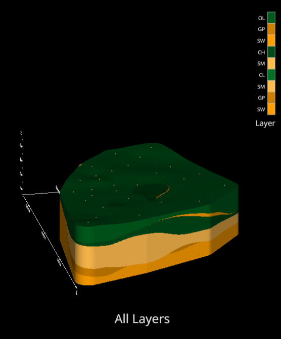
This example begins with the “resulting-stratigraphic-geologic-model.beginner.evs” application in the Earth Volumetric Studio Projects 2025.5 > Lithologic Geologic Modeling folder. This model has 9 geologic layers, and the upper 8 all have pinch outs. Here is the view of all the layers.

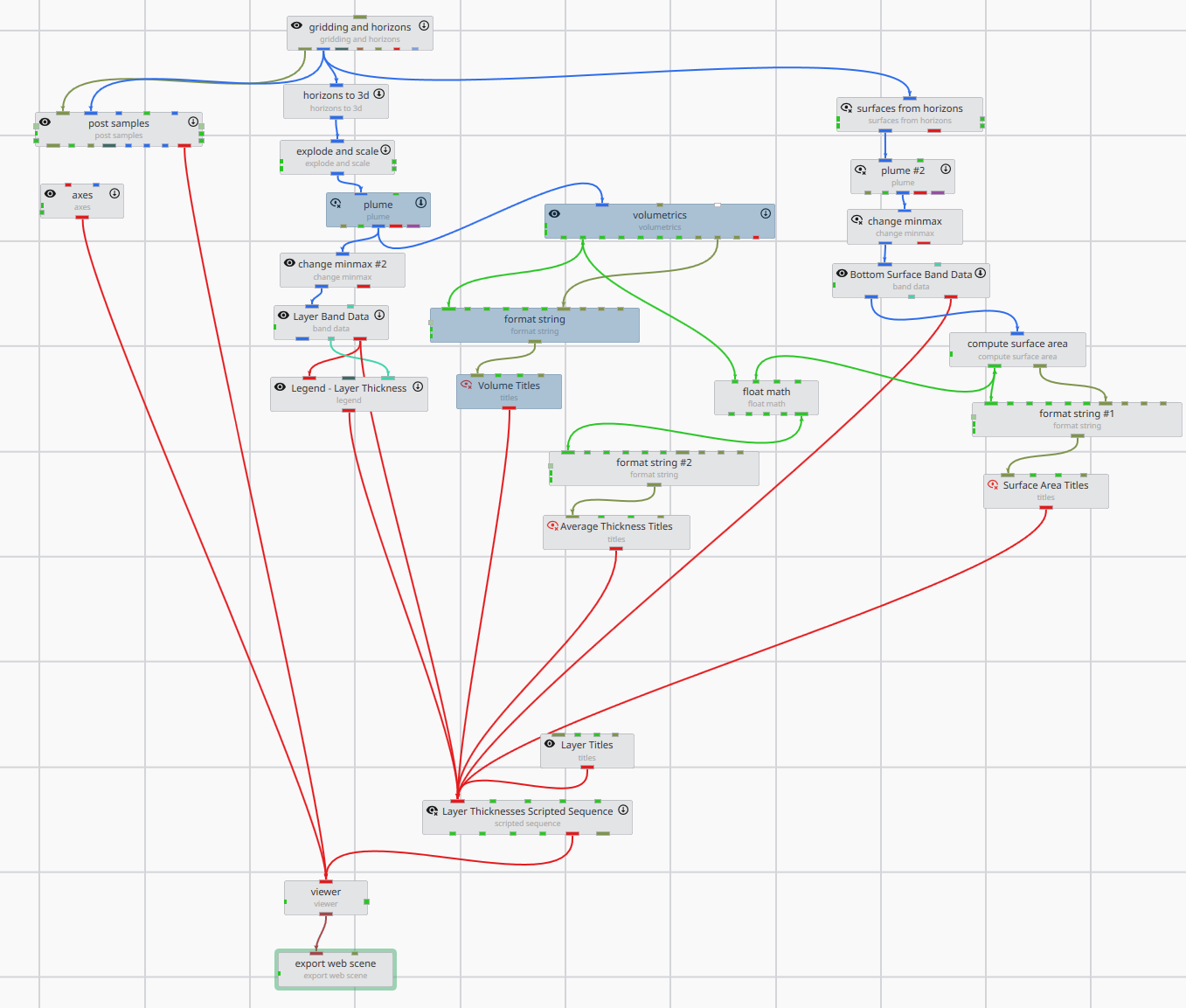
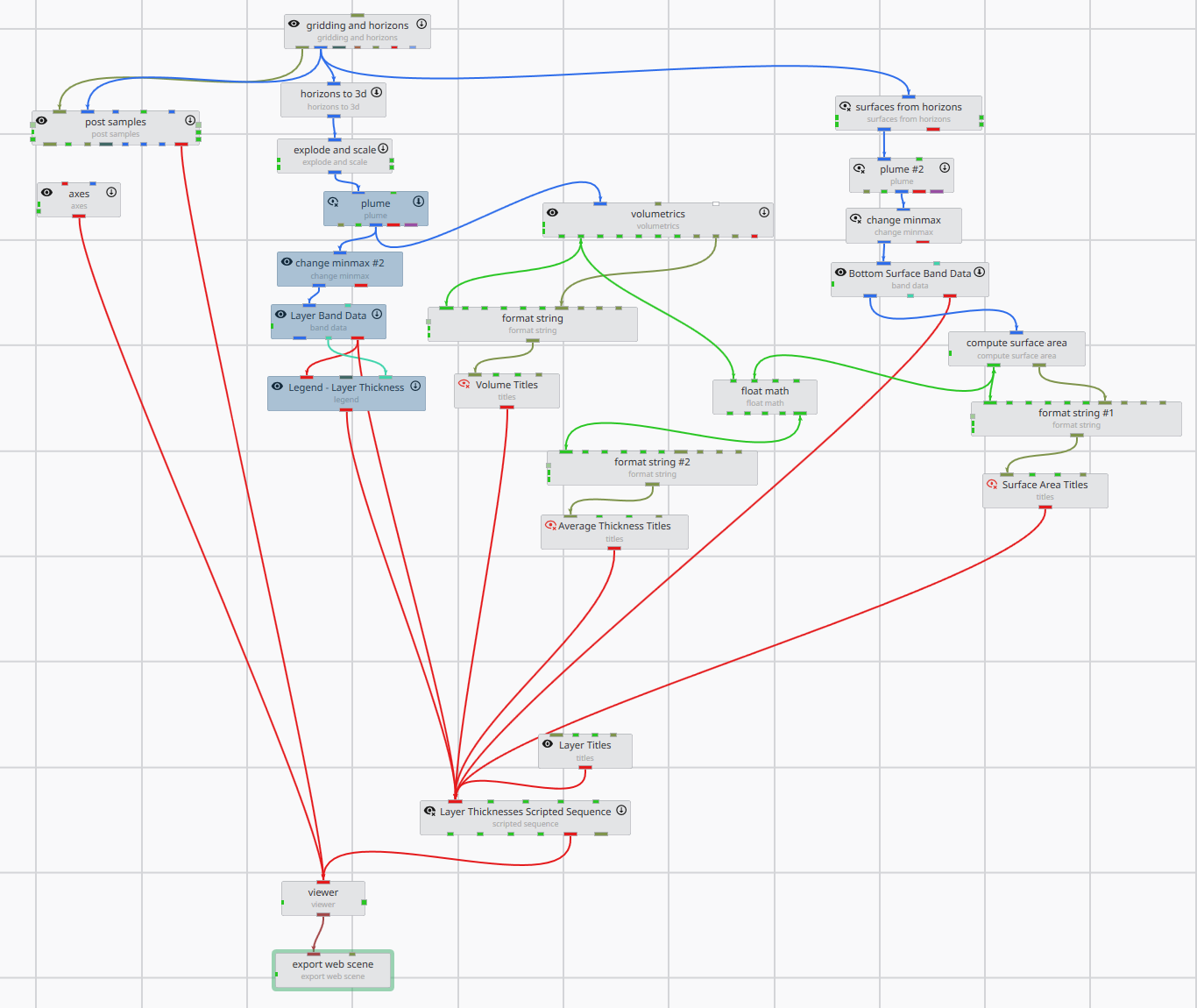
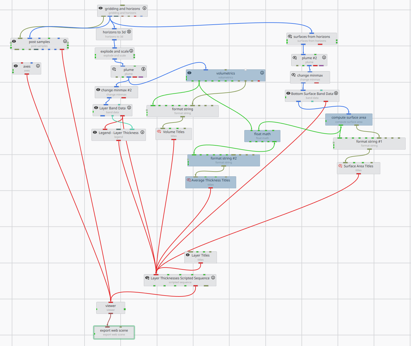
The following process chains were added to the model, as shown by the selected gray models in the images below: 1) a chain of modules running from explode and scale to calculate the volume:

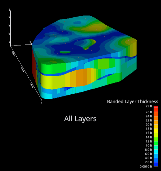
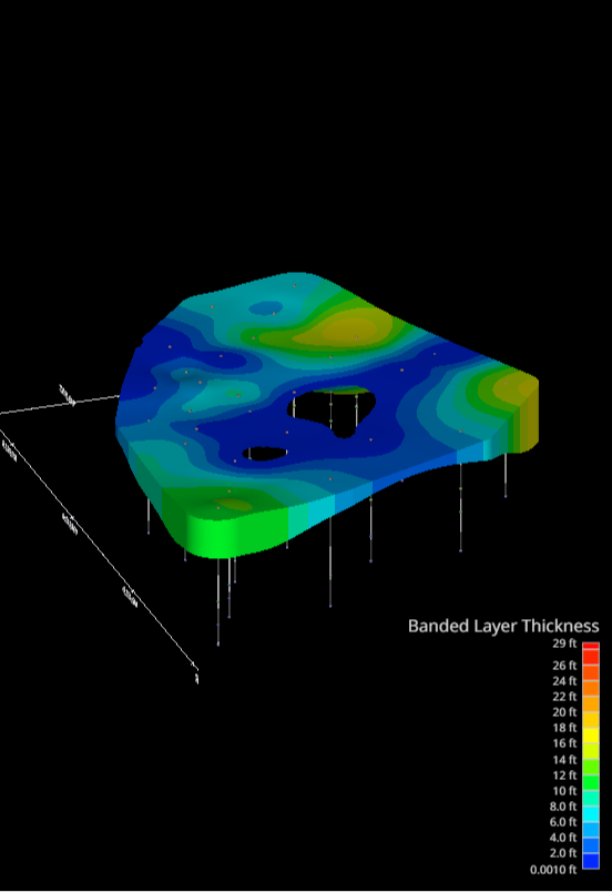
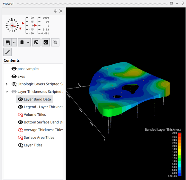
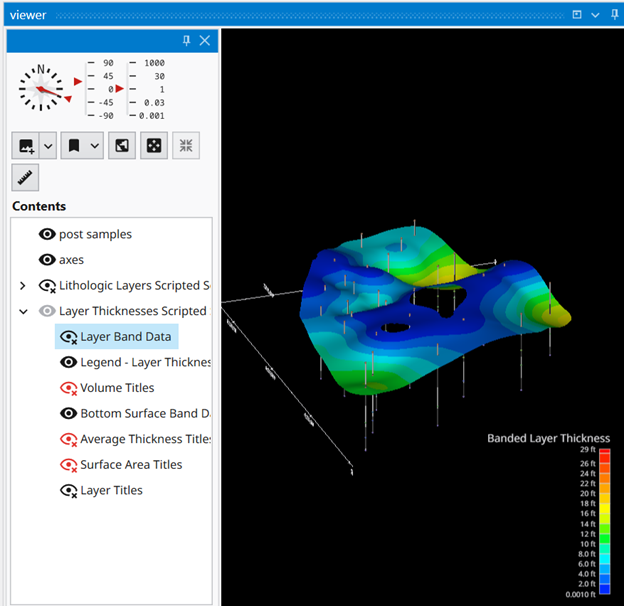
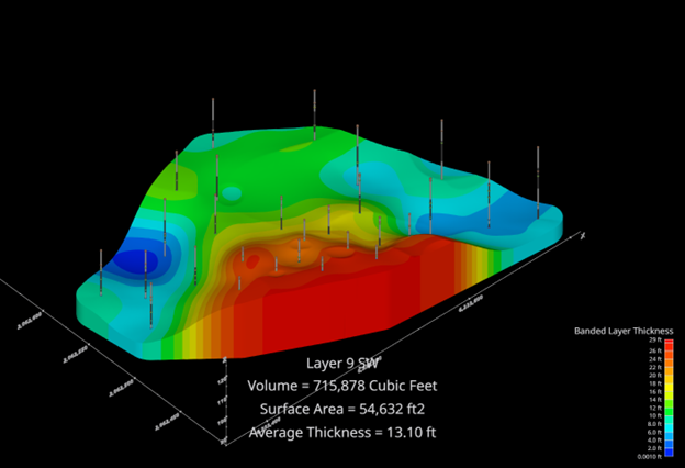
2. a chain of modules to color the layers by thickness bands:

…which looks like this:

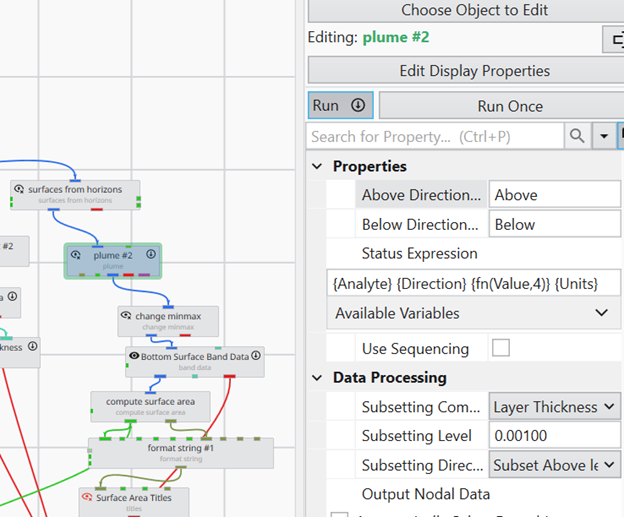
3. A chain of modules to calculate the surface area of each layer:

4. A computation chain that divides the volume of the layer by its surface area to calculate the average thickness:

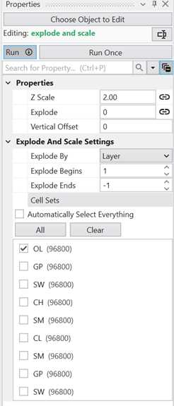
In order for the calculations for each layer to be correct, there are some key points that must be set properly to ensure the correct volume for a given layer is being divided by the correct surface area. For the volume chain, the explode and scale panel is used to select the layer. This is straightforward, as there is only one box for each layer:

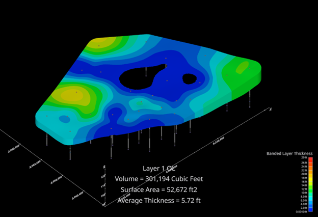
…which shows the top layer:

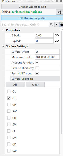
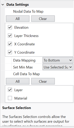
For the surfaces from horizons module, the selections must be chosen as follows to make sure you are getting the correct surface for your calculation. Here is what the panel looks like:

Note that there are two surfaces at the top for OL, because the top layer always has the ground surface and the bottom surface. All surface boxes below the OL layer select THE BOTTOM surface of the layer chosen. Note that Data Mapping needs to be set “To Bottom” to make sure you are getting the correct layer thickness data passed down the chain for subsequent calculations. You can check that you are selecting the correct layer bottom by toggling on/ off the volumetric “Layer Band Data” to see the surface below that is being used for the calculation:

You will also want to always set the Layer Thickness to the same value as you progress through each layer as it may change; in this case it is set to 0.001:

For the float math volume, the formula is simply N1 / N2, where N1 is the total volume passed from the volumetrics module, and N2 is the surface area passed from the compute surface area module.

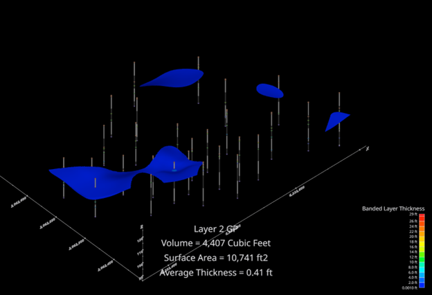
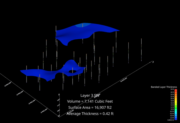
The resulting screenshots and calculation values are shown in sequence below.

Download the EVS Application

Published July 2025 - Based on EVS Version 2025.6.0

You are likely to encounter the requirement for 508 Compliance for some aspects of your work in the near future, if you haven’t already. Most U.S. Government agencies are required to make their websites and publicly accessible documents 508 compliant. For PDF files, whether or not they contain 3D Media, compliance is designated PDF/UA, for Universally Accessible.

If you are asked to make EVS outputs or a report with EVS modeling results 508 compliant this Tip will be relevant to you.

First, I need to disclose that this topic does not supplant the need for 508 accessibility expertise. Our goal is to provide guidelines which address the most fundamental accessibility requirements and suggest one path to meet them. You must appreciate that there are three levels of compliance (A through AAA) and EVS outputs, by their nature cannot fully meet them all.

These requirements attempt to address the needs of disabled persons meeting one or more of the following nine categories:

1. Without Vision
2. With Limited Vision
3. Without Perception of Color
4. Without Hearing
5. With Limited Hearing
6. Without Speech
7. With Limited Manipulation
8. With Limited Reach and Strength
9. With Limited Language, Cognitive, and Learning Abilities

In the case of PDF documents, including ones containing 3D media (Adobe’s term for interactive 3D content), we enhance the accessibility of the PDF by taking the following steps

• Layout your document including images, videos, and 3D media with a logical order.
• Ensure that PDF Accessibility Tags allow for navigation of the document in its intended order.
  • Though all content (headers, captions, paragraphs, links, images, videos, and 3D media, etc.) are required to be tagged, to meet PDF/UA standards, Adobe acknowledges that 3D Media cannot be tagged as of August 2024.
• Ensure that images, videos, and 3D media contain Alternate Text
• Ensure that images, videos, and 3D media have adjacent links to a detailed text description (e.g. Long Description) of what that media contains and represents.
  • Ensure that a link at the end of the detailed text description returns the user back to the relevant image, video, or 3D media.

Published May 2024 - Based on EVS Version 2024.3.0

I hope that all of our users have embraced C Tech Web Scenes (CTWS files) as their primary method to publish their EVS modeling results. C Tech Web Scenes have dozens of advantages over 4DIMs and all users should be aware that in the near future, the ability to create 4DIM files will be permanently dropped from EVS.

With that preamble, this topic will focus on the factors that affect the size of your CTWS files and the actions you can take to minimize that size.

You might wonder “Why should I care about the size of the CTWS files?”

• The simple answer is that smaller files are faster and easier for your clients. Whether you are:
  • Sending the files in emails
  • Placing them on a site for download, or
  • Embedding them on your company website
  • The client needs to download the file and the bigger it is, the longer that will take.
• Bigger files are also more taxing for the computer or device your client may be using. This can make everything sluggish.

What makes your CTWS files Large?

There are many things that affect the size of your CTWS files:

• Model size: The size of your models affects the size of the CTWS.
  • The product of you X-Y-Z Grid resolution determines the number of nodes and cells in you model. This directly affects the size of CTWS files.
  • The content of your application affects the size in various ways:
    • Lithologic models use grid smoothing which can dramatically increase the number of nodes and cells beyond what was in the input grid.
    • Annotation modules such as CAD, Shapefiles, Aerial Photos, etc. add to the model size
    • For example, the axes module defaults to 3D extruded text. Each character can have hundreds of nodes and the total size of axes can be significant.
    • Every module with a red output port which is connected to the viewer adds Objects to the CTWS Table of Contents and therefore adds to the model size.
    • The image used in overlay aerial can add size to your CTWS more than all other objects in your Table of Contents
    • The addition of any object with lines will automatically turn off the ability to Optimize Output. This can have a dramatic effect because optimization employs compression which can reduce the size of CTWS files by as much as 90%.
      • axes
      • external edges
      • isolines
      • 3d legend (note legend is ok because it is converted to a 2d image.)
      • CAD or Shapefiles with lines
      • Streamlines
      • Line fonts

Two items in particular can have a dramatic effect:

1. The image used in overlay aerial can add size to your CTWS more than all other objects in your Table of Contents
2. The addition of any object with lines will automatically turn off the ability to Optimize Output. This can have a dramatic effect because the compression inherent in Optimization can reduce the size of CTWS files by as much as 90%. However, the modules below are among those which can have lines in their output objects. Many of these can be converted to tubes instead of lines, but the items in red cannot be fixed in this way.
   • axes: The only alternative is the direction indicator module
   • external edges
   • isolines
   • 3d legend (legend is ok because it is converted to a 2d image)
   • CAD or Shapefiles with lines
   • Streamlines
   • Line fonts: (use TrueType fonts instead)

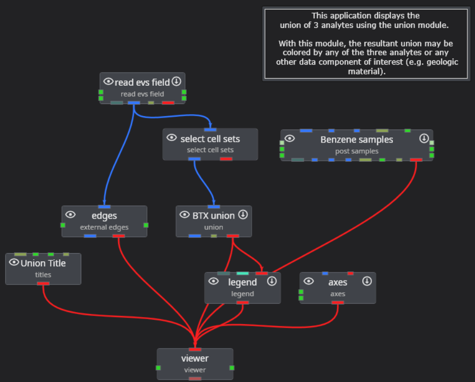
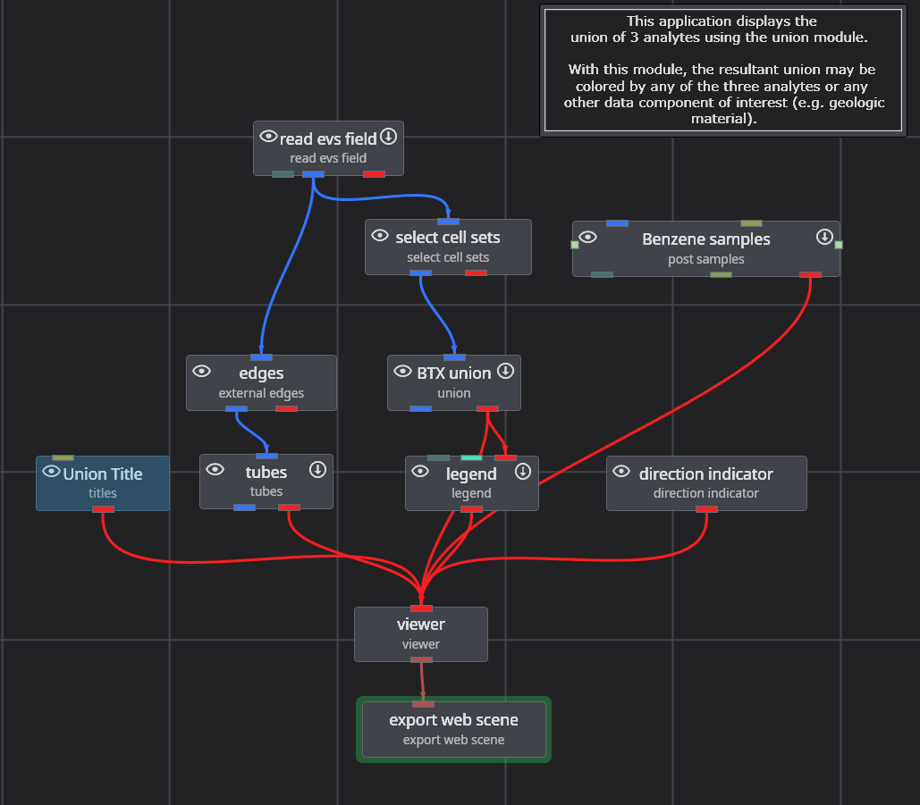
For this topic I’m going to use one of the Studio Project applications: Earth Volumetric Studio Projects 2024.1 > Analytical (Contaminant) Modeling > fuel-storage-union-efb.intermediate.evs. The application has these modules:

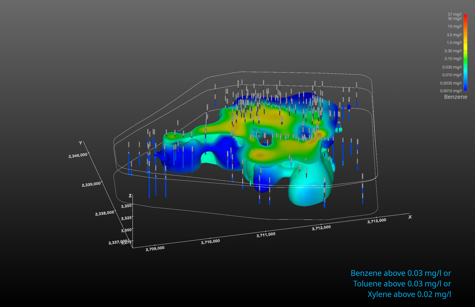
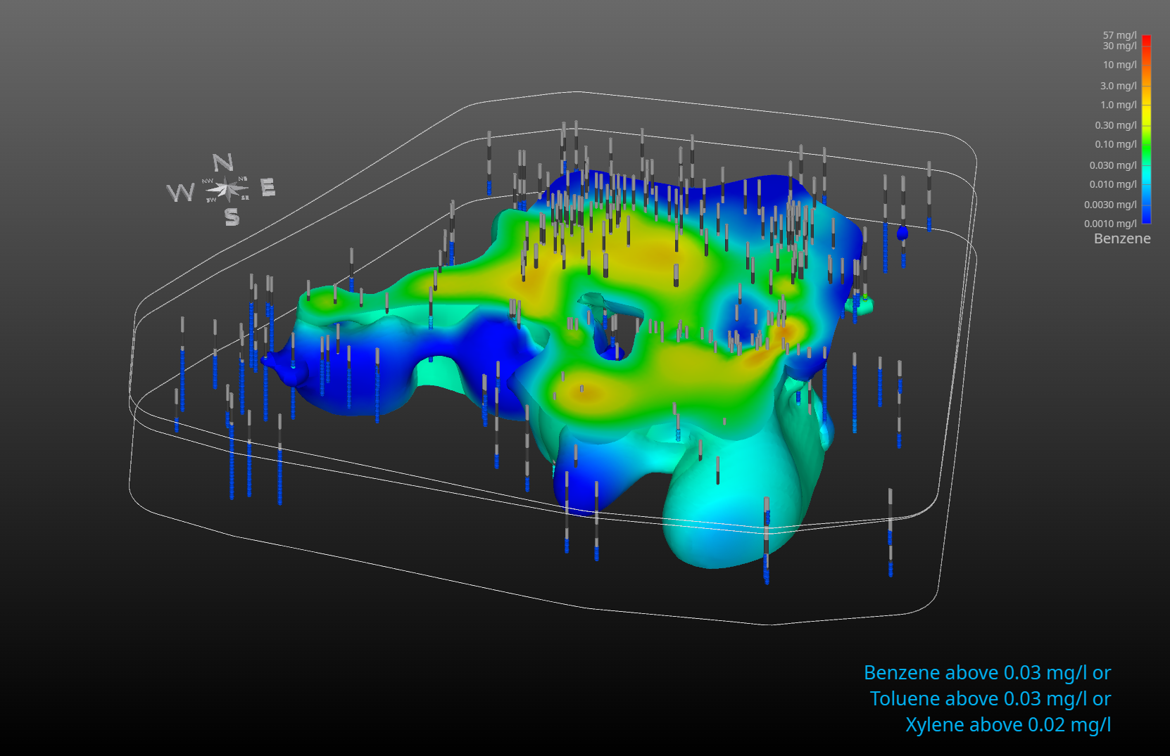
When I export the default version of this application as a CTWS file, the output looks like:

and the CTWS file cannot be optimized, resulting in a file size of 5.74Mb.

If we replace axes with direction indicator and pass external edges through the tubes module, the application becomes:

and the output looks like:

Now the CTWS file can be optimized, resulting in a file size of 727 kb (one-eighth as big).

Published May 2024 - Based on EVS Version 2024.3.0

BACKGROUND:

Based on our support inquiries, we know that many customers strive to include all aspects of a project into a single CTWS file. They may do this because of client or management pressure or because they cling to the potentially belief that more is always better than simple. Simple is often elegant and, more often, much easier for your client to use and understand. To this end, I have written this Tip to share some tricks to make your CTWSs clear and discoverable.

What helps to make a CTWS simple and discoverable?

• Descriptive and informative object (module) names in your Table of Contents (ToC)
• Use a shorter table of contents which is completely visible without scrolling

APPROACH:

One way to keep the Table of Contents succinct is to limit the scope of the CTWS. Your site may have multiple analytes, but unless you’re doing Unions or Intersections, it is easier for the client to understand how to navigate the CTWS if you restrict the content to be only one analyte. You would then use separate CTWS files for each analyte. In this way, all of your files are easier to use and understand.

Besides avoiding the risk of confusing your client, keeping your CTWS files small reduces the chance that a huge CTWS file will overwhelm your client’s modest computer that is normally used only for browsing or Word.

Below is our application to create a simple CTWS. There are no sequences in this example, but I am not suggesting that sequences need to be avoided. However, I would not recommend multiple sequences if the target user is likely to be more novice than expert.

The data for this application has eight unique analytes. These could be included in a single CTWS, but the end user will need to understand how to select one sequence to change the analyte and another to change plume levels or slice positions.

What makes this approach unique is that we will be able to quickly rename modules, and therefore the objects in the CTWS ToC instantly to create a highly customized ToC for each CTWS based on its analyte. We do this using the Python script below.

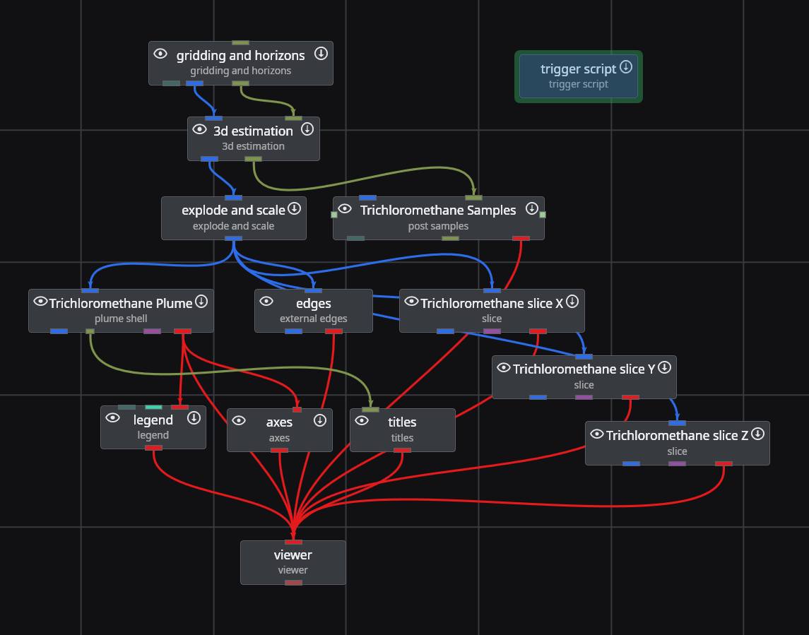
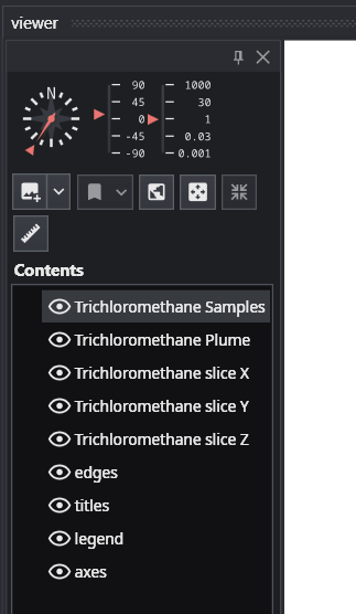
This script can be used for any application, with only needing to change the “analytes” list. We have 5 modules which include Trichloromethane in some of the module names. The corresponding ToC in EVS looks like:

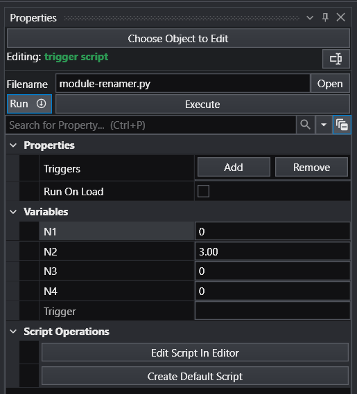
We reference this Python script in a trigger script module so it is included with our application, and so we can control the renaming using the N1 and N2 parameters. This avoids needing to edit the script.

With N1 = 0 and N2 = 3, we’re searching for Trichloromethane and replacing it with Benzene (the third analyte based on Python’s zero-based counting).

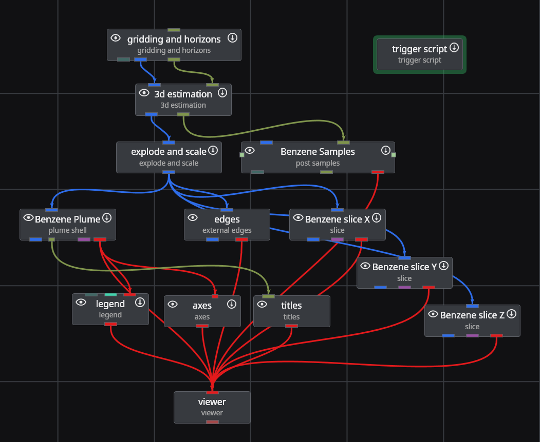
When we run this script, our application becomes:

You can easily enhance this script to control the Data Component (analyte in post samples and 3d estimation) as well as automatically writing the CTWS file.

Published April 2024 - Based on EVS Version 2024.3.0

I know that many of our users employ the distance to area module to cut away portions of their grid when the site boundaries are complex, but if you’re doing that without also using mask horizons, you’re missing a huge advantage with many positive consequences.

mask horizons provides a way to mask cells in the grid created by gridding and horizons. It can only be used directly after gridding and horizons and when used properly it removes regions of cells and their associated nodes from the grid, based upon an input surface, a.k.a. polygon mask.

• What does this do for you?
  • The masked regions are truly gone.
  • Those nodes and cells are not included in any analytic or geologic estimates downstream, which will reduce the computation times and memory footprint.

Let’s look at a dataset where mask horizons will cut your computation time and memory usage by over 80%.

In the “Lithologic Geologic Modeling” folder of Studio Projects you will find roadbase_lithology.pgf.

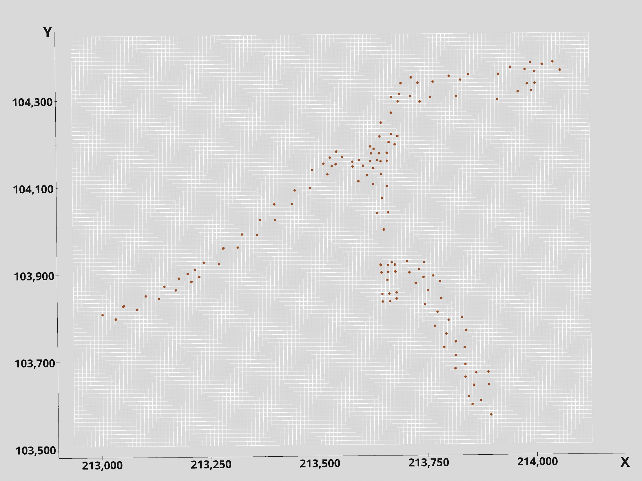
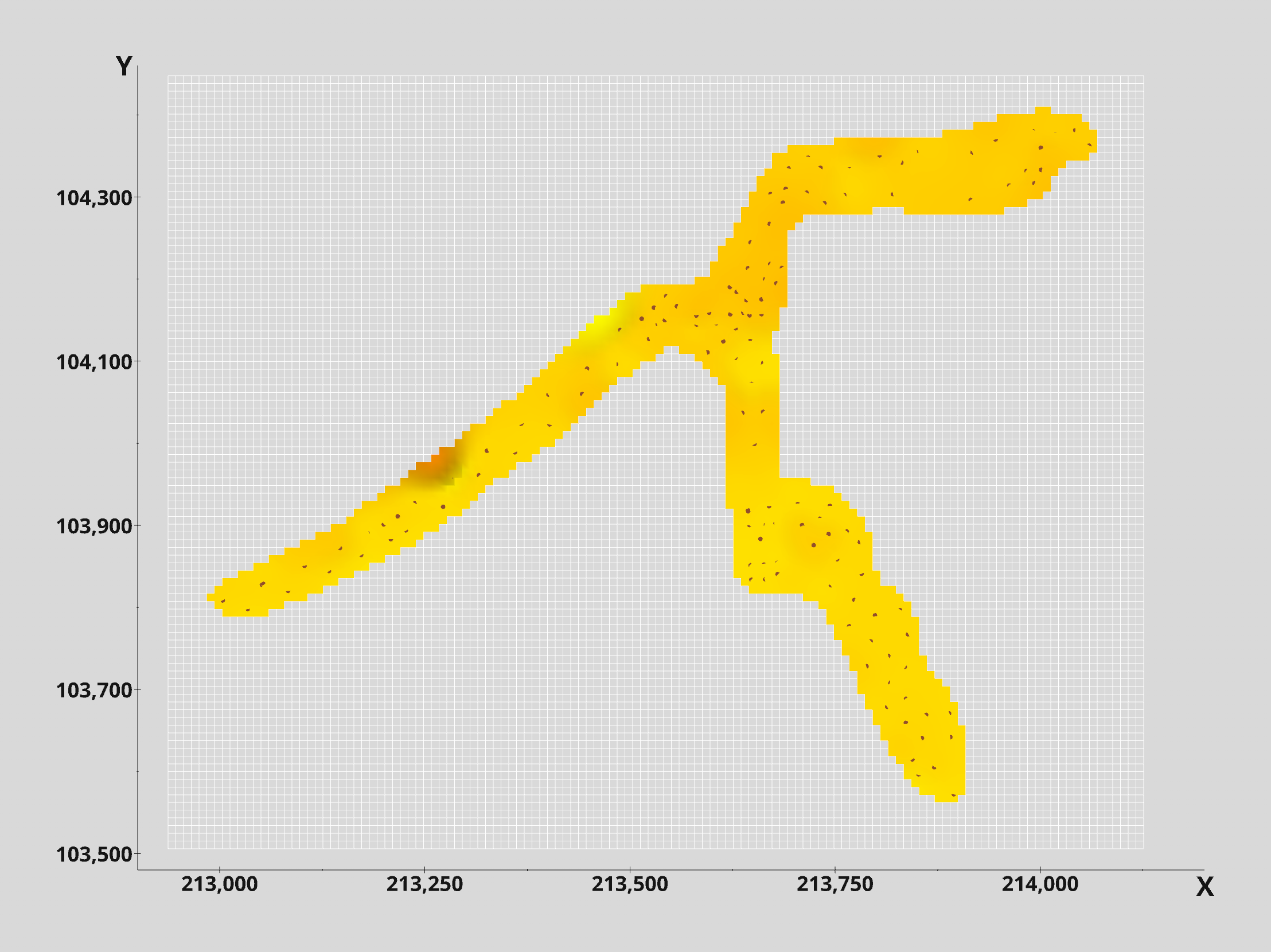
When we open that file in post samples and build a rectilinear grid in gridding and horizons (with a default 10% offset) we get this.

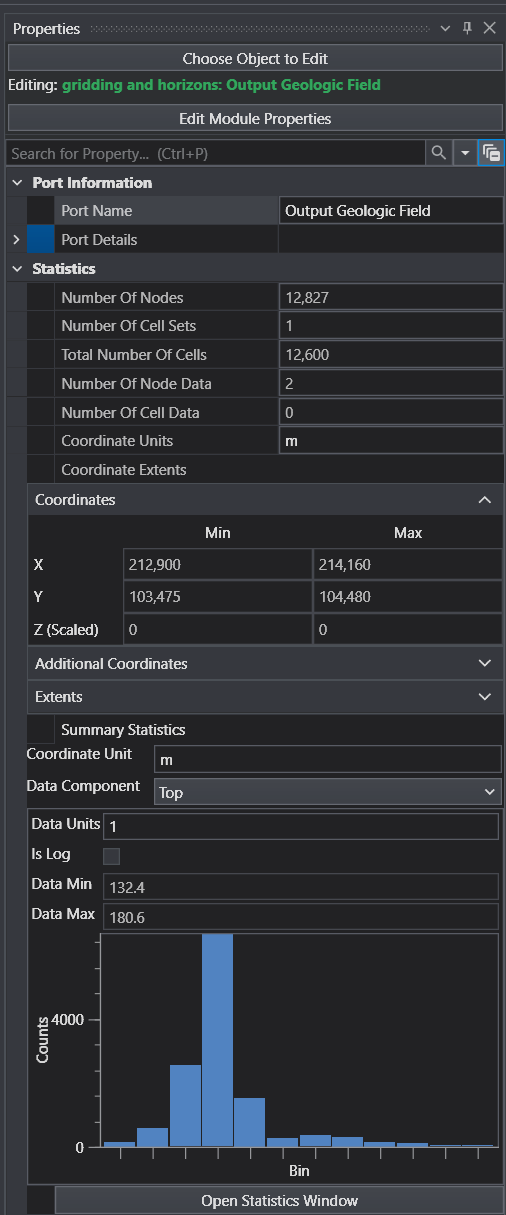
I used x-y resolutions of 127 x 101 to yield approximately 10 m square cells. The resulting grid has 12,827 nodes as we can see by double clicking on the blue output port of gridding and horizons. However, we can see that only a small portion of the grid area has data.

How do we confine the lithologic modeling to only those areas where there is data?

1. The first step is to create or use an existing polygonal area which is confined to the regions with borings.
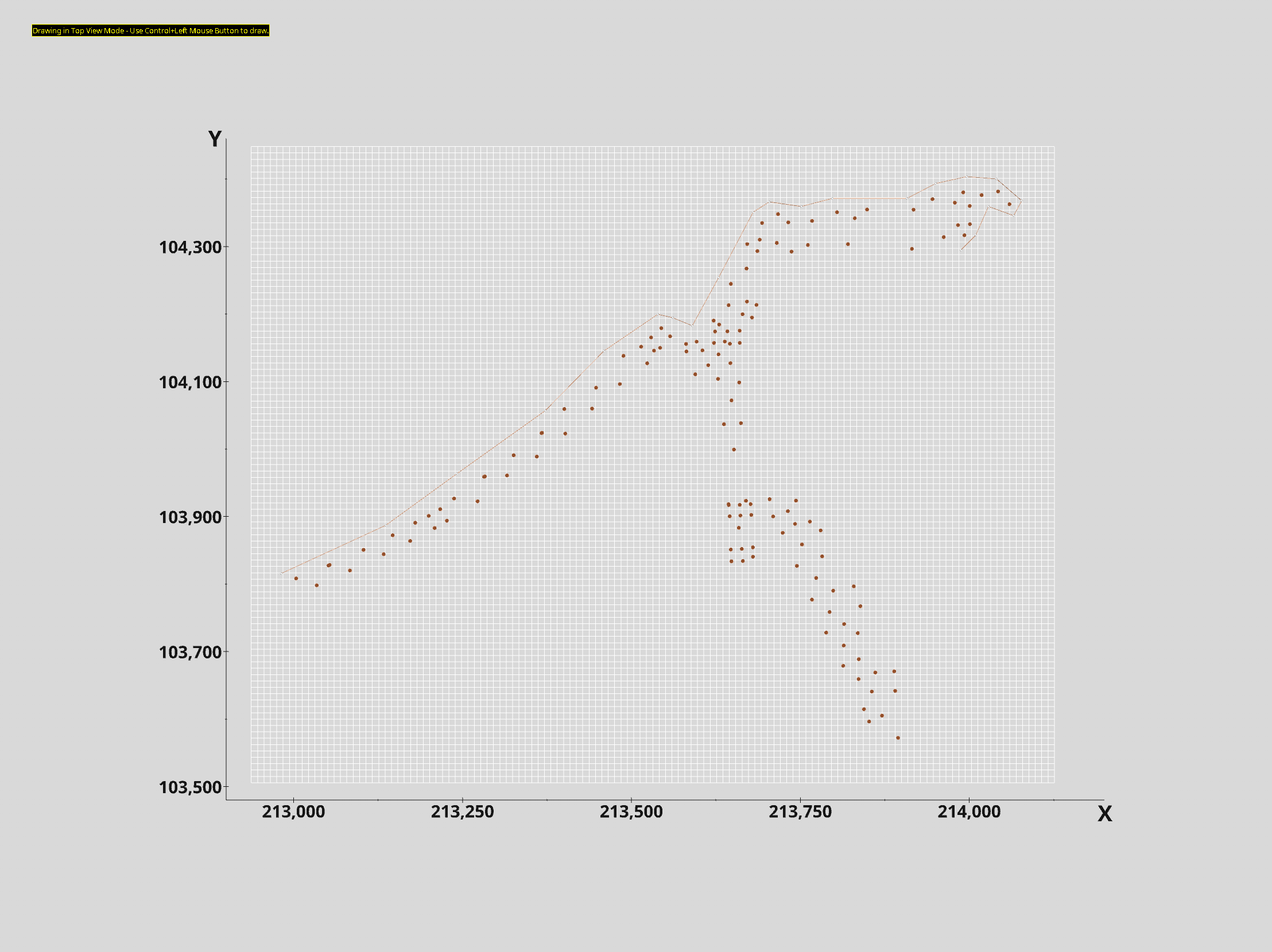
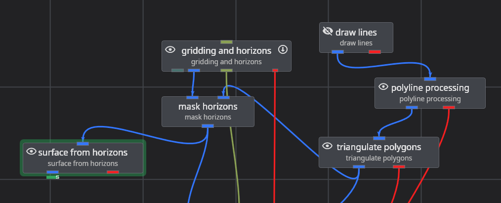
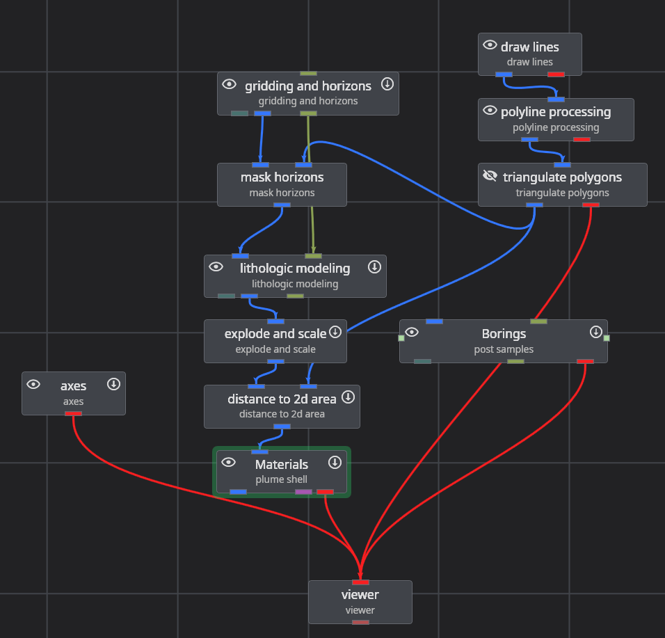
2. We’ll do this using the draw lines module together with triangulate polygons.
   1. We’ll use the Top View Mode “Drawing Style”.
   2. After adding ~25 points we see

With this approach, you choose how close you want to crop the grid to the data. In this case I’m staying close and that requires more points in my polygon boundary.

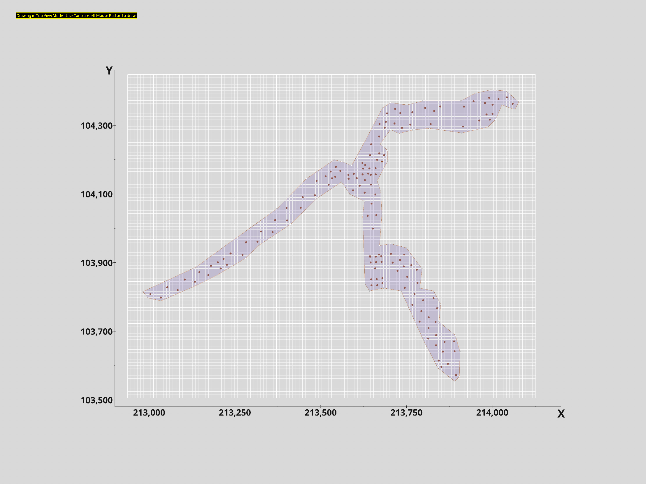
When your starting and ending points are close to each other, click the CLOSED toggle to close your boundary. This yields:

If we connect draw lines to triangulate polygons we get this:

Note: I’ve made the polygon transparent so we can still see the borings.

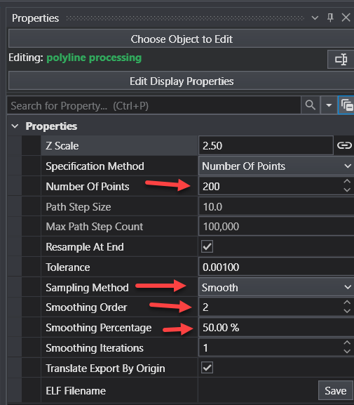
There is nothing wrong with this polygon, but I prefer a smoother boundary without the sharp corners. We can easily get this using the polyline processing module. Try these settings as a good starting point to give us a much smoother boundary.

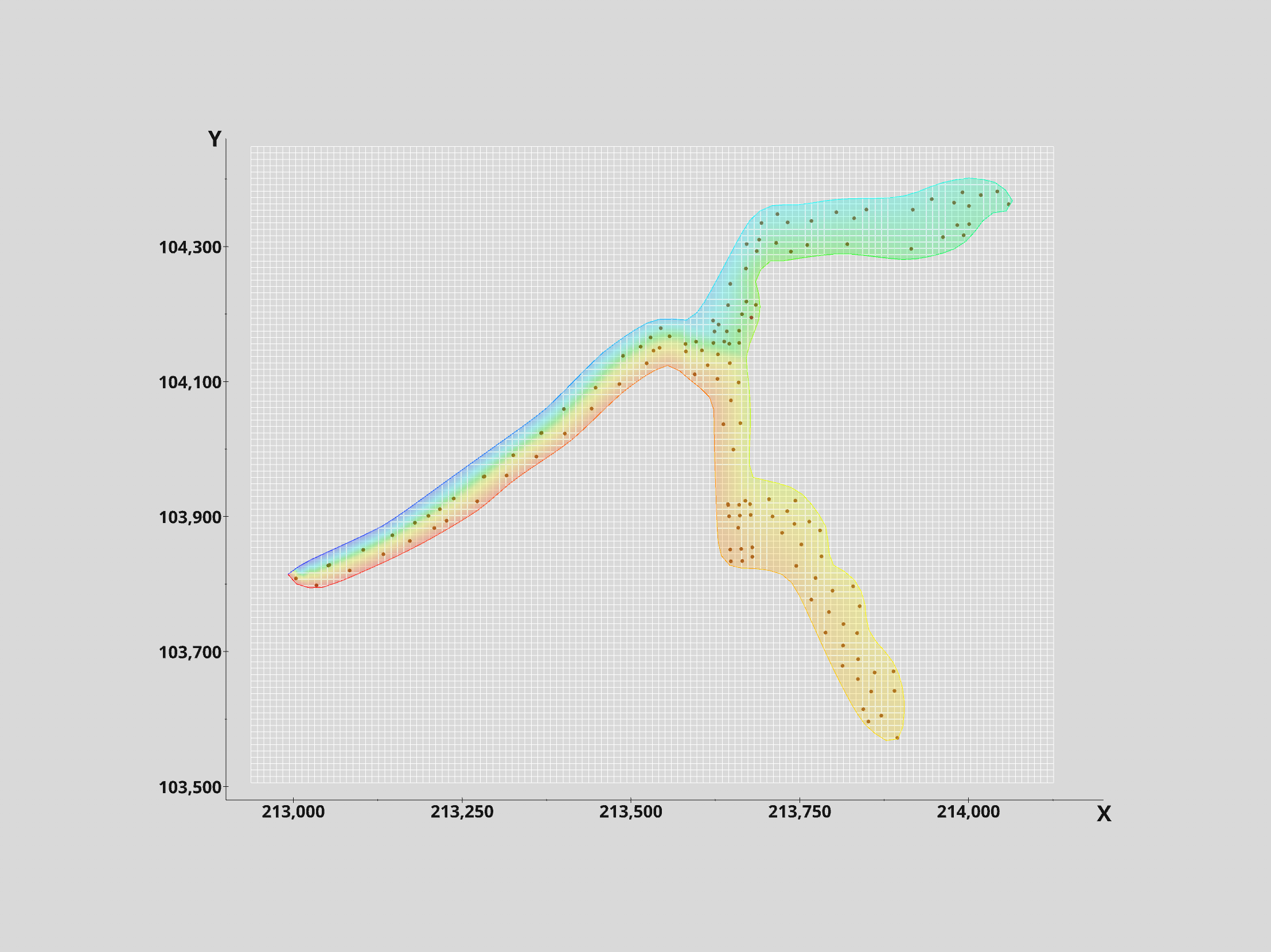
Note that the colors of the polygon changed because the smoothed lines have data corresponding to the node number. This allows us to see where we started (blue) and where we ended (red).

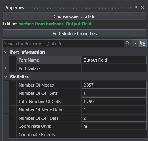
If we want to see how much we’ve reduced the original grid which had 12,827 nodes, we’ll need to grab another module: surface from horizons and double click on its blue output port to see our new grid’s statistics:

With only 2,057 nodes we’ve reduced the original grid by 84%!

You should be thinking “Why can’t I just use the blue output port of mask horizons? The answer is that it will still show the original number of nodes. That is because the masked nodes are only flagged (as NULL) for later removal by downstream modules.

You might also wonder if an 84% reduction in the 2D grid will still be an 84% reduction in the 3D grid. That answer is YES!

So what does our grid actually look like? Is it smooth like our polygon?

No, it is not smooth. It is Lego-Like because mask horizons marks cells for removal (or NULL treatment), so it is chunky at the resolution of our grid. However, this lego-ish grid created with the default settings of mask horizons will fully include all cells that even touch our smooth polygon. This ensures that we can later create a smooth boundary.

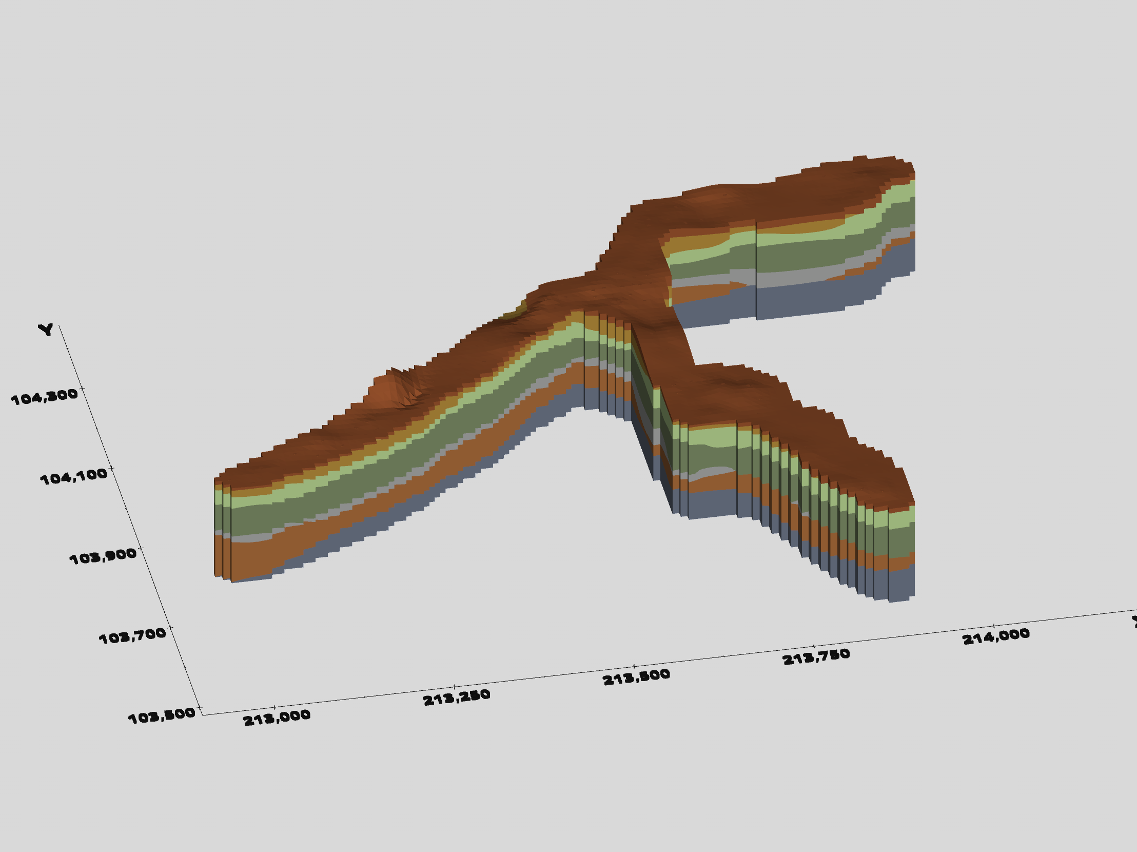
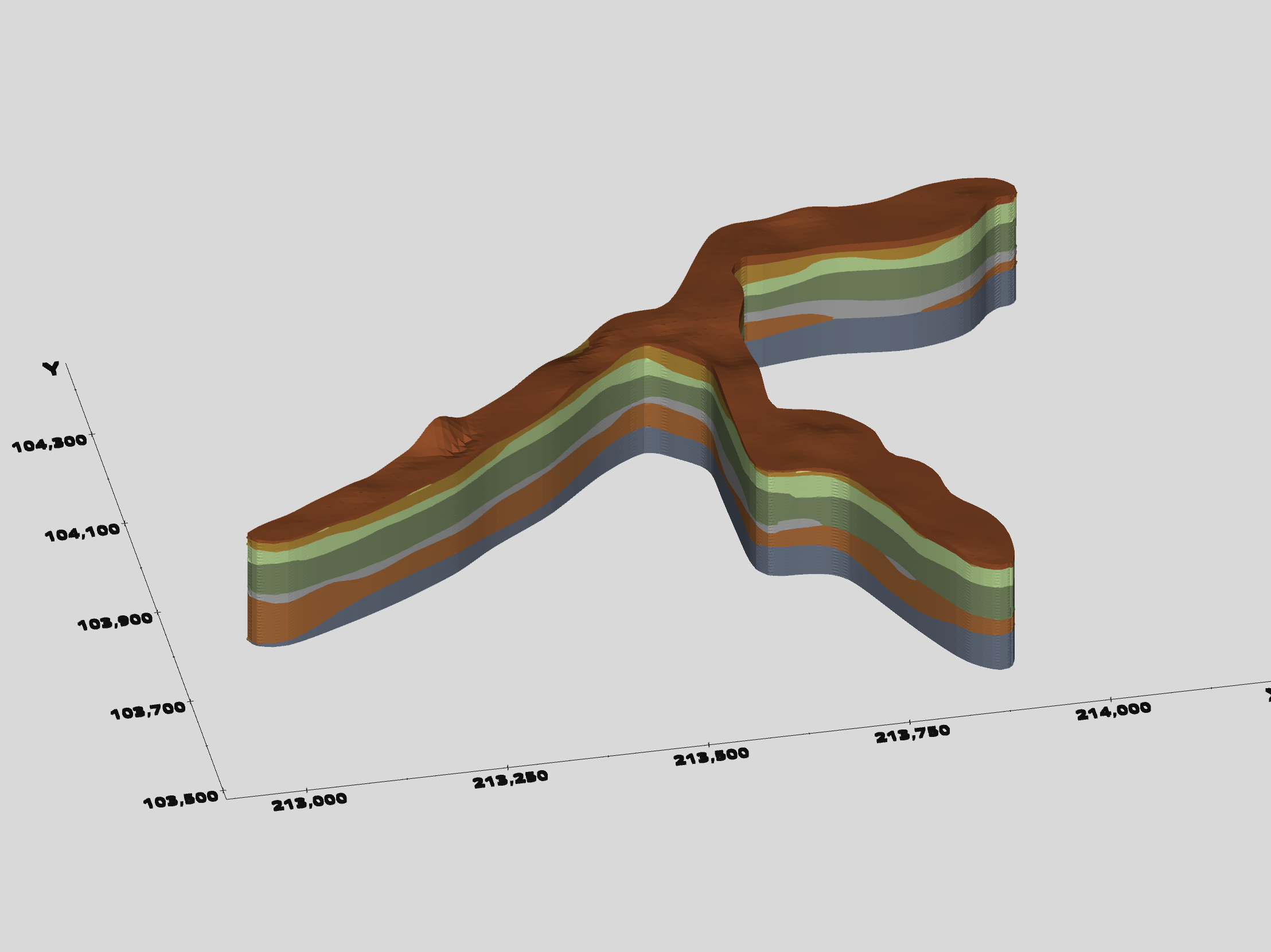
So, when we run the lithologic modeling module the 3D model will have lego-like boundaries

Our application to model this data has evolved as shown below. This has been saved for you as

roadway-lithology.mask-horizons.evs

Note that we’re still using distance to area to give us a smooth boundary.

You might wonder if the final model would look any different if we never used mask horizons, and the answer is YES!

However, the run time would be more than 6 times longer!

Published March 2024 - Based on EVS Version 2024.3.0

Application Bloat: Applications which, by design or due to inexperience or laziness, evolve beyond 50 modules fall into my definition of Application Bloat. With our current technology spearheaded by modules like scripted sequence, this is unnecessary. Over the years of technical support requests, I haven’t seen any 100+ module applications that could not be made more functional and have 70-90% fewer modules if you follow the advise below.

Recommended Development Stages:

1. BASE MODEL: When you complete the gridding, geology and initial analyte estimation, save this work and the resultant field with write evs field as a .EF2 file. You can then use read evs field to quickly get back to this model and in the process, replace all of those modules including explode and scale which is build into read evs field.

   1. Efficiency Trick: When you create your base model and save the .EF2 file, consider creating two versions!
      1. After you followed the guidelines in the EVS Training Videos to build a model with sufficient grid resolution to properly represent all of your data, and have saved the .EF2 file and application, make a second Coarse version of your model.
      2. If you use half as many nodes in X, Y & Z for the coarse model it will have one-eighth as many nodes and cells. This means that during your development stages, most everything you do will be nearly 10 times faster!
      3. But how do you use two versions of your model? It is built into the read evs field!

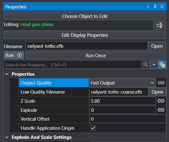
         1. In all of your read evs field modules, there are two file Open buttons for the two classes of input files: Highest Quality and Fast Output and a selector to choose between them (which you should leave linked!). The “Filename” is your fine model and the “Low Quality Filename” should be your coarse model. Leave Output Quality linked (as shown) and choose between these two options using Step 2.

            

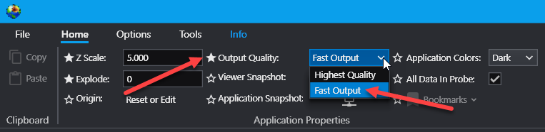
         2. On the home tab, the primary Output Quality selector is located and it is also available in Application Properties. As long as you don’t break the link in any of your read evs field modules, all of them will switch between Highest Quality and Fast Output with a single selection in either place. These two figures were captured at the same time and you can see that both reflect Fast Output.

            

2. FOLLOW ON STAGES: Save each application stage with a unique naming convention as below, but don’t forget to save with revision numbers as each stage evolves:

   1. ACME-Butte-Model.evs
   2. ACME-Butte-Revealed.evs
   3. ACME-Butte-Layers-Plumes.evs
   4. ACME-Butte-Roads.evs
   5. ACME-Butte-Final.evs

3. Need to Update: For any needed changes to the field (grid, geologic data, new analyte data), you merely return to the Base Model stage and recreate the .EF2. If you (backup and) overwrite your original .EF2 files, when you open your later stage applications they automatically be updated.

Your subsequent stage applications should focus on the steps below and when you embrace this order and paradigm, you’ll find that you avoid over complicating your application before that detail is needed.

1. Subsetting: How do I reveal the inner nature of the data?
2. Visualization: How best can I convey this information?
3. Annotation: What minimal enhancements will make the data more understandable?
4. Polishing and optimizing outputs for final client delivery.

When you have multiple analytes, don’t be lazy and include them by duplicating large branches of your application.

1. Use the techniques in this sequential subset (advanced training video) to handle any number of analytes with just a couple additional modules. This one trick can lead to a 90% reduction in required modules.

Summary on Bloat: If you choose to stick with 100+ modules applications, you face the greatest risk of loss and you have the most to lose!

Published March 2024 - Based on EVS Version 2024.3.0

BACKGROUND

My EVS Project Evolution

• Regardless of your level of expertise, my EVS applications often evolve in a non-linear fashion, but can benefit from a more structured approach. My initial effort is always understanding the data. The questions I am seeking to answer are:
  • What do the data sets, as a whole, represent?
  • What kind of grid suits my project best?
  • What type of geology am I dealing with?
  • If there is analytical data, what is the story I want to tell?
• Once I understand my data, I create my models and select the subsetting and visualization options which best tell my story.
  • I am frequently trying something and later changing or refining.

RULES TO MINIMIZE THE RISK OF LOSING HOURS OF WORK.

During all stages of your EVS project development, you need to employ a methodical process of saving your work. However, there are important steps that if followed, will minimize the risk of losing valuable time (and sanity).

• RULE NUMBER ONE: Save your application with a NEW name whenever you’ve made a significant change.
  • The obvious question is what is significant?
    • This is a personal definition that only you can answer.
    • For me it is ~15 minutes of real work.
  • Therefore, I strive to save my work with a new name every 15 minutes or whenever I make big changes which involves module additions or deletions.
    • What is a new name? I just add a dash and a revision number to my initial naming convention.
    • If my project is Roadrunner-blood-spill.evs then my first revision is Roadrunner-blood-spill-1.evs
• RULE NUMBER TWO: For full protection, you must regularly re-open your recently saved EVS revisions.
  • This is the only way to detect if some recent action on your part caused an instability in your application which could render your application unable to be loaded.
  • Once you understand the consequences of your application becoming unstable, especially if you lack functional back-up revisions, you will hopefully take this advise more seriously.

WHAT ARE THE SIGNS OF APPLICATION INSTABILITY.

These are a few of the things you may encounter which should signal you that your application is unstable. Please note that there are few ways to repair this condition, so the actions I recommend both above and below are critical. This is definitely a situation where prevention is more powerful than any available cure.

1. Worst Case: The worst thing you may encounter is that your application will not load. This means that the last time you saved, your application was already unstable. Pay attention to the signs below for instability and try to avoid saving, but in all cases don’t save over a known working revision!
   1. Empty Application Option: The only possible solution when this happens is to move (or copy) your application to a new folder, away from the data files referenced in the application.
      1. You may then be able to open this “empty” application.
      2. Work from Top-Down and one-by-one read your data files to try to find the cause of the instability.
      3. As you successfully execute branches of your application, save your application with a new revision name.
      4. Note: If the empty application cannot be opened, there is no other recovery option.
2. Application Unresponsive: If you find that your application is not responsive, it may be unstable.
   1. Don’t jump to this conclusion too quickly. If there is activity in the Output Log, this will make the application seem to be unresponsive, but it is actually BUSY. Busy is very different than unresponsive.
   2. An unresponsive application will typically not allow you to open a module’s properties. If the Output Log doesn’t show any activity, and a double-click on any module (or output port) in your application will not open its properties, your application is unstable. Saving the application is likely not useful and may not even be possible. But if you save it be sure not to save over a working version.
3. Application Stuck in Execution (a.k.a. Busy): If you find that your application is not responsive and the Output Log is active but not making progress, your application may be stuck.
   1. Again, don’t jump to this conclusion too quickly. Some modules may run very slowly with large datasets. Others have stages of their outputs that can take time and do not show progress. Examples are the smoothing process of lithologic modeling and while writing CTWS files with export web scene.
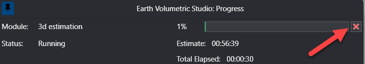
   2. Termination Option: If many minutes pass without progress, some modules have a Terminate button which may work.
      1. Be aware that it may take a few minutes for the termination of the process to complete, so have some patience. Obviously the more work you may lose if this fails, the more patient you should be.
      2. If termination is successful, you’ll want to check your modules settings and verify that there are not problems with the modules input data file. Both can cause long run times.
   3. Stuck: If the execution is truly stuck, which is indicative of it being in an infinite loop, there will not be anything you can do other than to close EVS. If EVS is unresponsive to the Window close [X], you’ll need to use the Task Manager to close it.
      1. There are two possible solutions in this case.
         1. If the fault is your data, fix the file and reopen your application.
         2. If the fault is settings in the offending module, use the Empty Application Option above.

WHAT ARE THE POTENTIAL CAUSES OF APPLICATION INSTABILITY.

Unfortunately, our users continue to find new ways to destabilize their applications or make them lock-up. However, we do see common threads among these problems and below you will find a description of the types of things you may be doing that increase your risks.

1. Application Bloat: Excessively large applications are the most commonly problematic and generally represent the greatest investment of time. In Optimized EVS Applications we offer guidelines which we’re confident will reduce the number of modules in your application and help you avoid instabilities.

2. Summary: If you choose to develop 100+ module applications, you face the greatest risk of loss and you have the most to lose!

3. Problem Data: Problems with your data can result in application instability. These tend to fall into two categories.

   1. Malformated Data: If you use C Tech’s export tools to create your data files, it is unlikely that your file will be malformatted, but it is still possible if their are certain non-standard characters in your Excel source file(s).
      1. Be very careful if you are manually editing or creating your data file.
      2. If you follow my recommendations above, you’ll be encountering this problem at a stage where your application is already saved and is quite simple.
   2. Unusual Data: I must acknowledge that among our thousands of software users we do encounter a few data files each year which are not malformatted but are problematic because of their nature and our software.
      1. Past examples of this are polylines or surfaces with zero-length edges resulting in redundant-coincident nodes.
      2. We consider this a software bug and endeavor to make our software robust enough to handle these problems, but we cannot plan for something we haven’t seen and can’t imagine.
      3. The Empty Application Option tends to work in these cases if you can’t just fix the file and re-open the application.

Published March 2024 - Based on EVS Version 2024.3.0

Bookmarks provide a quick and easy way to control your EVS application and they provide important control over your C Tech Web Scenes as well. They can control one or all of the following:

1. The view (Azimuth, Inclination, Scale, Roll, etc.) in the viewer
2. The Visibility and/or Opacity of all modules in the application which are connected to the viewer
3. The selected State of all Sequences in your application.

Why Use Bookmarks

• Bookmarks in EVS
  • Bookmarks can only be created (saved) in EVS and their primary purpose is to provide more control over C Tech Web Scenes
  • However, this does not mean that they are not incredibly useful in EVS.
    • The ability to save and recover the visibilities of all objects, set a view, and/or set all sequence states can help with your development and refinement of your application.
• Bookmarks in C Tech Web Scenes
  • Your goal as the EVS modeler should be to Tell the site’s story.
  • Bookmarks are a powerful tool that allows you to do that with a power and fidelity previously not possible.

What Can Bookmarks Do?

• Bookmarked Views (a.k.a. camera orientations) are Saved Azimuth, Inclination, Roll, Scale & Center
  • The Center which was last set in EVS will be the center.
    • It is not necessarily the center of the apparent view because an “apparent” center has no true 3D coordinate.
  • Selecting a view will set the camera orientation in EVS or Web Viewer to the saved settings.
  • EVS allows you to save any number of views. Please note that these will be affected if your model’s extents change which is why Bookmarks should be created when your application is mature.
    • By default, Views are name by Azimuth and Elevation: Azi 200 / Inc 18, however, YOU SHOULD ALWAYS RENAME BOOKMARKS to be more relevant to the end user, such as “Closeup view of Storage Tanks”
• Bookmarked Visibilities are collections of every module’s Visible and Opacity properties
  • Each visibility is the associated Visible and Opacity properties of all modules connected to the viewer at the time the visibility is saved.
  • LIMITATIONS: Our 3D Scene Viewer provides the ability control the visibilities of individual cell sets (e.g. geologic layers) within the objects, however, these cell set visibilities cannot be bookmarked in EVS.
  • The Visible and Opacity properties of modules which are added after saving a visibility are not controlled, so it is advisable to save visibilities only after your application is mature.
  • Visibilities only save object visibility and opacity. Parameters such as plume levels or slice positions are not saved.
  • The Visible property in group objects reflects the visibility of each object connected to the group.
    • Turning Visible on or off turns on or off the visibility of all objects connected to the group.
    • You cannot change the opacity of a group object.
  • Advanced visibility options: EVS you can set any object’s visibility to be On, Off, Locked or Excluded
    • Locked objects are On, but cannot be turned Off in C Tech’s 3D Scene Viewer
      • This is useful for items like a company’s Logo or other critical features you always want to remain visible.
    • Excluded objects are effectively not written to the CTWS. It is identical to disconnecting from the viewer in EVS.

Bookmarked States

• You can also save the selected State of all sequences in your model.
• Bookmarks do not control the state of individual sequences, but rather save and control the state of all sequences.
• Possible Unintended Consequences:
  • If you save the states of all sequences in EVS, but also include bookmarked Views and Visibilities to focus on one aspect of your model.
  • Even though you may only intend to control a sequence within the focus of this bookmark, the currently selected State of all sequences will be saved.
  • This means that if the end-user of the CTWS has changed other sequence states, those will be affected when the bookmark is played.
  • The only way to exclude specific sequences is if those sequences do not yet exist in your application when you save the bookmark.

How To Create Bookmarks

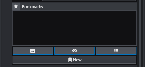
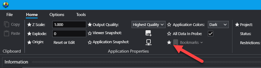
Bookmarks are created in Application Properties (if their visibility is ON). Below is the Bookmarks controls in Application Properties. Note the three buttons which are shown on (highlighted in blue). From left to right, these are Views, Visibilities and Sequence States.

You can choose to have any bookmark change just one or all of these action classes. It isn’t always ideal to have bookmarks control all three actions. It is up to the Application Creator to decide on the optimal functionality.

When you are ready to create a new bookmark:

• Decide what actions you want and set the View, Visibilities and/or States in EVS to those conditions.
• Turn on the appropriate action buttons
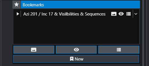
• Press the New button to see the new bookmark with Default naming

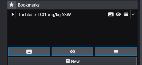
Our default naming includes the Azimuth and Inclination (if the first action button is ON) and also tells you that it is also controlling Visibilities and Sequences. However, this name is only an appropriate name if only View is controlled. You should rename this Bookmark to be as informative as possible, such as Trichlor > 0.01 mg/kg SSW.

TIME TO RENAME YOUR BOOKMARK

It is more important to properly name your bookmark than any other action you may take. Put yourself in the position of your client, the end-user of the C Tech Web Scene you will be delivering. What good is a bookmark if the client cannot ascertain its purpose and function?

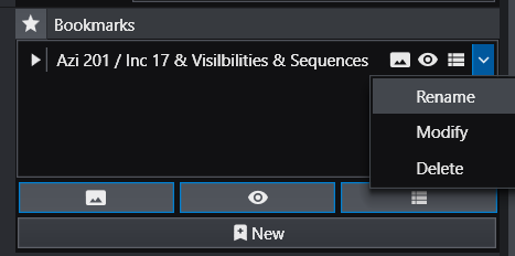
To rename it, click on the down arrow to the far right and select Rename.

HOW TO PLAY BOOKMARKS

Bookmarks are saved and played (used) in the Application Properties window, but they must be turned ON in the main Ribbon as shown below:

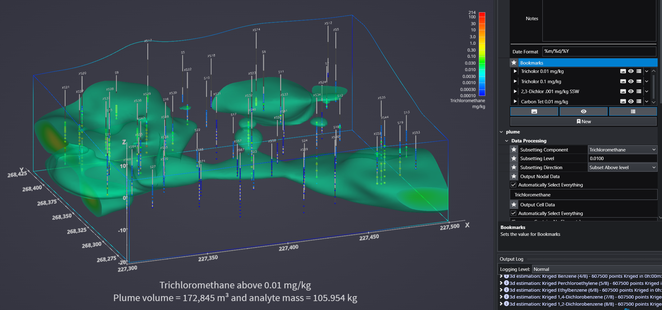
Bookmarks are played (applied) in Application Properties (if their visibility is ON). The example below has 4 bookmarks, and each is set to control the View, Visibilities and Sequence State. Note that each has a play icon (white triangle) on the left. Clicking Play triggers the functionality of the bookmark to be applied to the application in EVS. Similarly, if a CTWS file is saved for this application, all four bookmarks will be included.

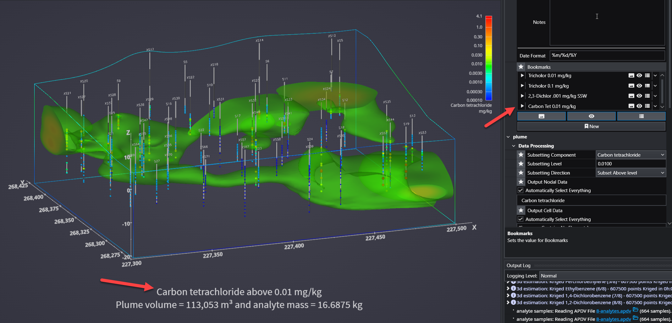
Clicking on the last of these bookmarks produces this:

This is complicated to explain and difficult to completely understand. Let me start by saying that if we build a rectangular (rectilinear) grid with 10m cells, where the nodes fall exactly on the 10s, 20s, etc. (233000.0, 233010.0, 233020.0,…) and we use any of our interpolation methods, the elevations we compute at the even 10s, will be exactly the same as if we build the same grid with 5 meter cells, adding additional nodes at the centers of each of the original 10m cells.

Does that mean that the 5 meter grid is more accurate?

The only places where the finer grid can be more significantly more accurate is where we have noisy data that it can honor. As we move away from the data, we will have relatively smooth surfaces (possible slopes and even convex or concave curves) but the elevations at the middle of the 10 meter cells will be extremely close to the estimated values on our 5 meter grid. Only the addition of random, noisy data in areas will create a surface that has complexity which allows the finer grid to honor the data better.

The question I ask myself is if we see patterns of small hills and valleys, with varying distances (frequencies) of these bumps, should our estimation method try to simulate these bumps as we move further from the data? The answer to this question is ABSOLUTELY NOT.

We cannot know how the distances between this random surface structure will change. If we add these bumps, we are likely to put a bump where there should be a valley and a valley where there should be a bump. This could double or quadruple our errors and create a much poorer model. As we move away from measured data we want an estimate that will create a surface that will be the average of the bumpy surface, passing through the middle of the hills and valleys.

2. That is correct. We would need to have a grid where all surfaces are adaptively gridded using the X-Y coordinates of all horizons. This is not impossible, but is much more complicated and it is unlikely we would try to do this initially. Also, as discussed above, it doesn’t likely help that much!

Attached is an application which I believe will better explain the issue of accuracy. However, first we need to acknowledge that there are two “ACCURACY” issues involved.

The customer was concerned about the ACCURACY of the gridded surface to precisely match the data values.

I’ve explained this and demonstrated that adaptive gridding can provide a surface which exactly matches the data at the X-Y locations.

I believe it is more important to understand the ACCURACY of ESTIMATED surfaces to match ACTUAL horizon elevations.

If the layer thicknesses which affect their piling installations are important, and if those pilings will not be exactly where they measured elevations, this is what really matters.

As I tried to explain, the accuracy to which C Tech’s estimated surfaces will actually match the real horizons depends on the nature of the surface and the amount and distribution of actual measurements.

The more data that is collected the better the surface is defined.

The smoother and more well behaved the surfaces are, the less data is needed.

Surfaces with quickly changing slopes will need more data.

Finer gridded surfaces can provide closer matches at the measured locations.

Adaptively gridded surfaces can provide exact matches at the measured locations.

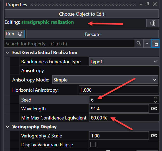
C Tech’s “stratigraphic realization” module provides a way to see possible scenarios (realizations) of what MIGHT exist in the real world. It uses the nominal estimated surface and computed standard deviations to create one possible “synthetic” horizon based upon two fundamental statistical parameters:

A random number generator “Seed”

The Confidence level you wish to have. A higher Confidence will generate greater deviations, but there will be a greater chance that the actual real-world deviations will not be greater than the realizations.

THE MOST IMPORTANT THINGS TO UNDERSTAND ARE:

WHERE THERE IS DATA, THE REALIZATION SURFACE DOESN’T MOVE. WHY?

We know the actual elevation.

Therefore, the Standard Deviation at that location is ZERO.

IF WE CREATE THOUSANDS OF REALIZATION SURFACES AND AVERAGE THEIR ELEVATIONS, WE WILL GET THE NOMINAL ESTIMATED SURFACE.

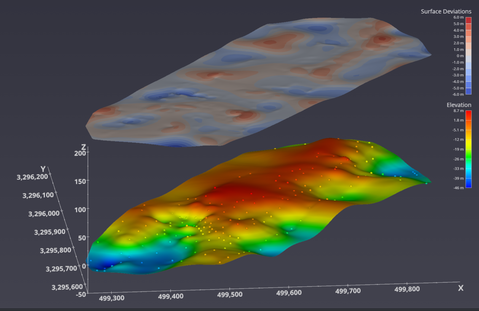
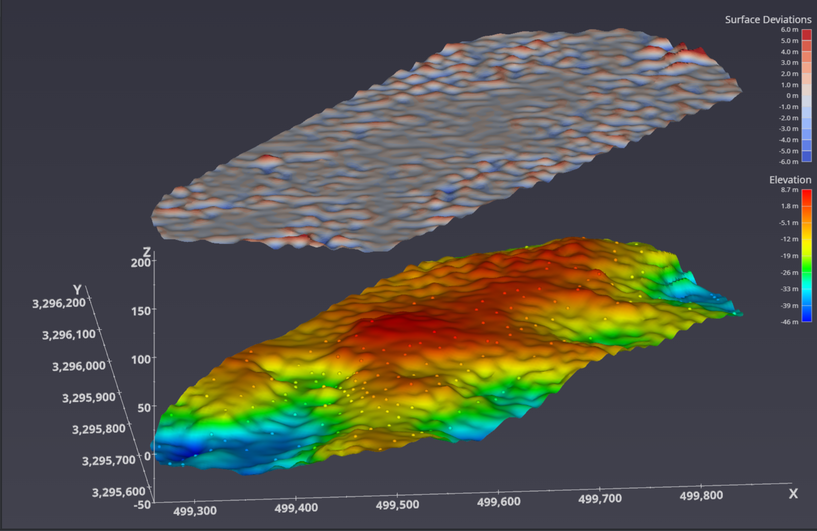
Once we have this Horizon Realization, we can compute how much it “deviates” from the nominal surface estimate. These deviations help to quantify the potential inaccuracies that might be encountered because of the Nature of the actual horizon and the quantity and distribution of measured data.

Your customer must understand that THERE IS NO PERFECTLY CORRECT (RIGHT) ANSWER.

You also might want to investigate the Wavelength parameter to see that the deviations might be high frequency or low frequency. For this dataset a wavelength of 15-20 is interesting because it is similar to the localized surface “bumps” caused by closely spaced samples that vary wildly in elevation.