Module Libraries

Module Libraries

EVS modules can each be considered software applications that can be combined together by the user to form high level customized applications performing analysis and visualization. These modules have input and output ports and user interfaces.

  • Map sparse data to surface and volumetric grids.
  • Create surfaces or 3D volumetric grids with lithology and stratigraphy.
  • Visualization functions for rendering models and data.
  • Quantification and statistical information.
  • Add axes, titles, legends, and other references to visualizations.
  • Extract subsets of grids or data for boolean operations.
  • Create data for subsetting or assessing proximity to surfaces, areas, or lines.
  • Read files containing grids, data, and archives.
  • Write files containing grids, data, and archives.
  • Create animated sequences from driven, scripted, or object-based state changes.
  • Simulations and vector data functionality.
  • Create or act upon grids and geometric primitives.
  • Transform grids into other coordinates or dimensionality.
  • Aerial photos and bitmap operations.
  • Work with time domain data.
  • A collection of utility modules.
  • Visualization and output of results.

See also: Legacy Module Naming — reference for old-to-new module name mapping.

Subsections of Module Libraries

  • 3d estimation

    Performs a three dimensional estimation of analytical data. Can also estimate analytical data sourced from other fields, or map data onto an external grid.

  • 2d estimation

    Performs a two dimensional estimation of analytical data. Can also estimate analytical data sourced from other fields, or map data onto an external grid.

  • cross validation

    Performs cross validation of estimation results.

  • gridding and horizons

    Create complex grids and estimate data into horizons.

  • analytical realization

    Perform Fast Geostatistical Realizations of analytical data.

  • stratigraphic realization

    Perform Fast Geostatistical Realizations of stratigraphic data.

  • lithologic realization

    Perform Fast Geostatistical Realizations of lithologic data.

  • lithologic assessment

    Perform assessment of lithologic data quality.

  • external kriging

    The external kriging will output both data and a grid in the simple GeoEAS format.

Subsections of Estimation

3d estimation

3d estimation performs parameter estimation using kriging and other methods to map 3D analytical data onto volumetric grids defined by the limits of the data set, or by the convex hull, rectilinear, or finite-difference grid extents of a geologic system modeled by gridding and horizons. The module provides several convenient options for pre- and post-processing input parameter values, and allows the user to consider anisotropy in the medium containing the property.

3d estimation also has the ability to create uniform fields, and allows the user to choose which data components to include in the output. Uniform fields require no geologic input and Adaptive Gridding must be turned off (otherwise the connectivity is not implicit).

The DrillGuide functionality produces a new input data file with a synthetic boring at the location of maximum uncertainty calculated from the previous kriging estimates, which can then be rerun to find the next area of highest uncertainty. There are no limits to the number of cycles that may be run.

Variogram Options:

There are three variogram options:

  1. Spherical: the default and recommended choice for most applications
  2. Exponential: generally gives similar results to Spherical and may be superior for some datasets
  3. Gaussian: notoriously unstable, but can “smooth” your data with an appropriate nugget. Without a nugget term, Gaussian is generally unusable. If Gaussian kriging is overshooting the plume in various directions, the nugget is likely too small; if the plume looks overly smooth, the nugget is likely too big.

The “Power Factor” is only used for exponential or Gaussian variograms. The default value of 3 is the most common value for exponential. For Gaussian, 2 is most common, though values from 0.1 to 3 are typically acceptable.

Advanced Variography Options:

3d estimation supports complex directional anisotropic variography. The variogram is displayed as an ellipsoid that can be distorted to represent primary and secondary anisotropies and rotated to represent heading, dip, and roll. Overall scale and translation are provided as visual aids to compare the variogram to the data, though these do not affect the actual variogram.

Ports

DirectionNameTypeDescription
InputInput Geologic FieldFieldThe main geologic field input for the module.
InputInput External GridFieldA field containing an external grid to use for the output. (Advanced Version Only)
InputInput External DataFieldA field containing external data to use instead of reading a file. (Advanced Version Only)
InputInput FilenameStringFile used to estimate analytical data.
OutputOutput FilenameStringFile used to estimate analytical data.
OutputOutput FieldFieldThe main output field with analytical data added.
OutputStatus InformationStringText containing the full status information output from the module.
OutputOutput ObjectRenderableA renderable object displaying the uncertainty sphere(s) and variography created by the module. Output even when Allow Run is off.
OutputAnalytical Grid DataRealizationInformation required for direct exporting of raw analytical grid data.
OutputInterpolation OptionsInterpolation OptionsInformation about the interpolation settings such as variogram parameters and number of points used in interpolation.

Properties

PropertyTypeDescription
Allow RunBooleanControls whether the module will run when applications are loaded or data changes. When on, the module runs when applications are loaded or the Execute button is pushed. When off, the module will not run unless Execute is pressed.
FilenameFileThe file containing the data to interpolate onto the created grid.
Data ComponentIntegerSelects which property value in the analyte file will be kriged. The default value of -1 results in kriging of all data components in the file.
ExecuteButtonForces the module to run. If pressed and the application saved, the module will run when the application is loaded.
Z ScaleDoubleThe vertical exaggeration to apply to the variogram and the uncertainty sphere.

Grid Settings

PropertyTypeDescription
Grid CoordinatesCoordinatesDefines the coordinate domain within the data set in which kriging will be completed. Min and Max values are only used when the Rectilinear option is selected.
X ResolutionIntegerThe number of grid nodes in the model horizontal domain.
Y ResolutionIntegerThe number of grid nodes in the model vertical domain.
Z ResolutionIntegerThe number of grid nodes in the model elevation domain.
Layers From GeologyChoice: Make Single Layer, Use all HorizonsUsed with the input geology port. Controls whether to create a single layer or a layer for each horizon.
Min Cells Per LayerIntegerThe minimum number of cells in the Z direction per layer. Used when proportionally gridding an input geologic grid.
Cells Per LayerIntegerThe number of cells in the Z direction per layer when not using proportional gridding.
Proportional GriddingChoice: Cells Per Layer, Proportional Z ResolutionWhen multiple geologic layers exist, apportions cells to layers in Z based on each layer’s average thickness, subject to the Min Cells Per Layer parameter.
Grid TypeChoice: Uniform or Structured Field, Irregular MeshThe type of grid to create for interpolation.
Adaptive GriddingBooleanRefines the grid automatically to place grid nodes at all measured data points, ensuring the output honors all measured locations exactly.
Adaptive Gridding LimitIntegerTurns off adaptive gridding when the number of sample points exceeds this value.
Adaptive Value PriorityChoice: Favor Min Values, Favor Max ValuesSpecifies the criteria for which sample to use for adaptive gridding when more than one sample is contained by the same grid cell.
Minimum Layer ThicknessDoubleThe smallest vertical height of each cell.
Reverse Surface HierarchyBooleanDefines layers starting from the bottom to the top.
Boundary OffsetDoubleCreates a domain larger than the input data along all three axes.

Data Processing

PropertyTypeDescription
Data ProcessingChoice: Linear Processing, Log ProcessingAllows the module to be run in either linear or log space.
Data ScalingDoubleA value by which all nodal data values will be multiplied before kriging.
Pre Clip MinDoubleAny nodal property value less than this number will be replaced during preprocessing.
Pre Clip MaxDoubleAny nodal property value greater than this number will be replaced during preprocessing.
Less Than MultiplierDoubleApplied when reading a file with values flagged with the ‘<’ character. Multiplies the file value by this multiplier.
Detection LimitDoubleAffects file values set with the ‘ND’ or other non-detect flags. The module inserts a value equal to (Detection Limit * Less Than Multiplier).
Post Clip MinDoubleThe smallest nodal value that will be present in the output data field.
Post Clip MaxDoubleThe largest nodal value that will be present in the output data field.
Auto Exponentiate External Log DataBooleanDetects if data imported via the External Data port has been log processed and exponentiates it, avoiding double log processing.
External DataMulti-selectSelects which data components from the External Data port to use for interpolation.

Krig Settings

PropertyTypeDescription
Estimation TypeChoice: Kriging, IDW (Shepard), IDW (Franke/Nielson), Nearest Neighbor, FastRBFThe method for interpolating file data onto the created grid.
ReachDoubleThe radial distance from any given model node that the module will look for data points. Setting to 0 causes the module to calculate a reach approximately two-thirds of the longest distance between any two data points.
Points In ReachIntegerThe maximum number of data points within the reach to consider for parameter estimation at a model node.
Octant SearchBooleanWhen selected, searching is performed for each of the eight octants surrounding the point to be kriged.
Use All PointsBooleanCauses the module to include samples up to the All Points Limit value. If the number of samples exceeds the limit, Reach and Points In Reach settings are used.
All Points LimitIntegerThe maximum number of points to use when interpolating. If there are more samples than this value, Reach and Points In Reach settings will be used.
Statistical Confidence ToleranceDoubleSpecifies the interval in linear space around the kriged model estimates to which the kriging confidence or uncertainty applies.
Statistical Confidence FactorDoubleSpecifies the interval in log space around the kriged model estimates to which the kriging confidence or uncertainty applies.
Min Max ConfidenceDoubleSpecifies the interval around the kriged model estimates to which the kriging confidence or uncertainty applies.
IDW PowerDoubleUsed with Inverse Distance Weighting. Greater values increase the influence of values closest to the interpolated point.
Variogram And AnisotropyVariogramControls the semi-variogram model and 3D anisotropy settings for kriging.

Time Settings

PropertyTypeDescription
Chem File Is Time DomainBooleanCauses the file to be read as a time file, with values interpolated first to the set date and then to the grid.
Specify Date By ComponentBooleanAllows the Data Component value to select a date, resulting in exact data at a date instead of an interpolated value.
Date For InterpolationDateThe date of interest. Used with the Interpolation Type to determine the value of a sample before interpolation onto the grid.
Analyte NameStringThe analyte name for date files.
Date Interpolation MethodChoice: Direct Interpolation Only, Interpolate Only, Interpolate and Extrapolate Beyond, Interpolate and ExtrapolateDefines how to interpolate when given unsampled times in a file.
TCF File NameFileThe output TCF file name. When the module runs, it loops through each component and creates an EFB file; the dates and filenames are added to the TCF file.
Create TCFButtonCauses the module to run in a loop, going through each component and creating an EFB file at that time. These EFB files are linked together in the specified TCF file.

Data To Export

PropertyTypeDescription
Auxillary Kriging DataMulti-select: Max Plume, Min Plume, Statistical Confidence, Standard Deviation, Statistical UncertaintySelects which kriging-derived data components to include in the output field on a node by node basis. Available when using Kriging estimation.
Geologic Nodal DataMulti-select: Layer Thickness, Depth, ElevationSelects which geologic data components to generate for the output field on a node by node basis. For structured grids, Layer Thickness is exported as cell data.
Geologic Cell DataMulti-select: Material ID, Geo LayerSelects which geologic data components to generate for the output field on a cell by cell basis.

Display Settings

PropertyTypeDescription
Uncertainty Spheres To DisplayMulti-selectSelects which uncertainty spheres to display. There is one sphere per analyte, each reflecting the location of maximum uncertainty for that analyte.

Variography Display

PropertyTypeDescription
Display Variogram EllipsoidBooleanDisplays the variography ellipsoid in the viewport.
Ellipsoid OpacityDoubleSets the opacity of the ellipsoid.
ResolutionIntegerThe resolution of the ellipsoid. Larger numbers create more detailed representations.
Ellipsoid ScaleDoubleScales the ellipsoid equally along each axis.
X OffsetDoubleTranslates the ellipsoid along the x axis.
Y OffsetDoubleTranslates the ellipsoid along the y axis.
Z OffsetDoubleTranslates the ellipsoid along the z axis.
Ellipsoid ColorColorThe color of the variogram ellipsoid.
Display Variogram LinesBooleanDisplays lines aligned with the variography ellipsoid.
Line ScaleDoubleA scalar that sets the length of the variogram lines relative to the scale of the ellipsoid.
Primary Ratio ColorColorThe color of the primary ratio axis line.
Secondary Ratio ColorColorThe color of the secondary ratio axis line.
Tertiary Axis ColorColorThe color of the tertiary axis line.

Drill Guide

PropertyTypeDescription
Create DG FileButtonRuns the module in a loop, creating a synthetic boring at the maximum uncertainty location until the Number Of Synthetic Samples is reached.
Synthetic Sample PrefixStringAllows the user to alter the prefix string for generated synthetic boring names.
Number Of Synthetic SamplesIntegerControls how many times drill guide will run.
Boring SamplesIntegerIndicates how many samples to create at each synthetic boring.
Target ConcentrationBooleanWhen selected, changes the location of the uncertainty sphere based upon the specified Target Isolevel.
Target IsolevelDoubleWhen Target Concentration is selected, this value is used to change the location of the uncertainty sphere.
User PointsCoordinatesManages points added to the grid for drill guide purposes to eliminate areas of high uncertainty that cannot be drilled, such as under a building.

2d estimation

2d estimation performs parameter estimation using kriging and other methods to map 2D analytical data onto surface grids defined by the limits of the data set as rectilinear or convex hull extents of the input data.

Its Adaptive Gridding feature further subdivides individual elements to place a “kriged” node at the location of each input data sample. This guarantees that the output will accurately reflect the input at all measured locations (i.e. the maximum in the output will be the maximum of the input).

The DrillGuide functionality produces a new input data file with a synthetic boring at the location of maximum uncertainty calculated from the previous kriging estimates, which can then be rerun to find the next area of highest uncertainty. The naming of the “DrillGuide©” file which is created when 2d estimation is run with all types of analyte (e.g. chemistry) files ends in apdv1, apdv2, apdv3, etc. There are no limits to the number of cycles that may be run.

2d estimation also provides special data processing options that allow it to extract 2-dimensional data sets from input data files containing three-dimensional data, and allows detailed analyses of property characteristics along 2-dimensional planes through the data set. The module also provides options to magnify or distort the resulting grid by the kriged value of the property at each grid node, and allows automatic clamping of the data distribution along a boundary offset from the convex hull of the data domain.

Variogram Options:

There are three variogram options:

  1. Spherical: the default and recommended choice for most applications
  2. Exponential: generally gives similar results to Spherical and may be superior for some datasets
  3. Gaussian: notoriously unstable, but can “smooth” your data with an appropriate nugget. Without a nugget term, Gaussian is generally unusable. If you find that Gaussian kriging is overshooting the plume, your nugget is likely too small; if the plume looks overly smooth, your nugget is likely too big.

Ports

DirectionNameTypeDescription
InputInput External GridFieldA field containing an external grid to use for the output. (Advanced Version Only)
InputInput External DataFieldA field containing external data to use instead of reading a file. (Advanced Version Only)
InputInput FilenameStringFile used to estimate analytical data.
OutputOutput FilenameStringFile used to estimate analytical data.
OutputOutput FieldFieldThe main output field with analytical data added.
OutputStatus InformationStringText containing the full status information output from the module.
OutputSurfaceRenderableA renderable object displaying the component surface.
OutputAnalytical Grid DataRealizationInformation required for direct exporting of raw analytical grid data.
OutputInterpolation OptionsInterpolation OptionsInformation about the interpolation settings such as variogram parameters and number of points used in interpolation.

Properties

PropertyTypeDescription
Allow RunBooleanControls whether the module will run when applications are loaded or data changes. When on, the module runs when applications are loaded or the Execute button is pushed. When off, the module will not run unless Execute is pressed.
FilenameFileThe file containing the data to interpolate onto the created grid.
Data ComponentIntegerSelects which property value in the analyte file will be kriged. The default value of -1 results in kriging of all data components in the file.
Data PriorityChoice: Maximum Values, Minimum ValuesAffects which samples are adaptively gridded.
ExecuteButtonForces the module to run. If pressed and the application saved, the module will run when the application is loaded.
Z ScaleDoubleThe vertical exaggeration to apply to the variogram, the uncertainty sphere, and the output surface.

Grid Settings

PropertyTypeDescription
Grid TypeChoice: Rectilinear, Convex HullThe type of grid to create for interpolation. Convex Hull creates a model with irregular boundaries defined by the extent of the measured data points.
Grid CoordinatesCoordinatesDefines the coordinate domain within the data set in which kriging will be completed. Min and Max values are only used when Rectilinear is selected.
X ResolutionIntegerThe number of grid nodes in the model horizontal domain.
Y ResolutionIntegerThe number of grid nodes in the model vertical domain.
Adaptive GriddingBooleanRefines the grid automatically to place grid nodes at all measured data points, ensuring the output honors all measured locations exactly.
Adaptive Gridding LimitIntegerTurns off adaptive gridding when the number of sample points exceeds this value.
Boundary OffsetDoubleThe distance in user units that the grid coordinate range for the kriging domain will be set outside of the actual coordinate range of the data.

Data Processing

PropertyTypeDescription
Data ProcessingChoice: Linear Processing, Log ProcessingAllows the module to be run in either linear or log space.
Data ScalingDoubleA value by which all nodal data values will be multiplied before kriging.
Pre Clip MinDoubleAny nodal property value less than this number will be replaced during preprocessing.
Pre Clip MaxDoubleAny nodal property value greater than this number will be replaced during preprocessing.
LT MultiplierDoubleApplied when reading a file with values flagged with the ‘<’ character. Multiplies the file value by this multiplier.
Detection LimitDoubleAffects file values set with the ‘ND’ or other non-detect flags. The module inserts a value equal to (Detection Limit * LT Multiplier).
Collapse MethodChoice: Max, MinThe method for extracting data within a depth interval when multiple samples exist. Duplicate samples at the same x, y, z coordinates are averaged first.
Distance To CollapseDoubleThe maximum distance in 2D that points will be considered coincident. Coincident points will be dropped depending on the Collapse Method.
Post Clip MinDoubleThe smallest nodal value that will be present in the output data field.
Post Clip MaxDoubleThe largest nodal value that will be present in the output data field.
Auto Exponentiate External Log DataBooleanDetects if data imported via the External Data port has been log processed and exponentiates it, avoiding double log processing.
External DataMulti-selectSelects which data components from the External Data port to use for interpolation.

Krig Settings

PropertyTypeDescription
Estimation TypeChoice: Kriging, IDW (Shepard), IDW (Franke/Nielson), Nearest Neighbor, FastRBF, Natural NeighborsThe method for interpolating file data onto the created grid.
Use GradientsBooleanUsed with Natural Neighbor interpolation. When on, gradients estimated at sample points improve the interpolation result.
ReachDoubleThe radial distance from any given model node that the module will look for data points. Setting to 0 causes the module to calculate a reach approximately two-thirds of the longest distance between any two data points.
Points In ReachIntegerThe maximum number of data points within the reach to consider for parameter estimation at a model node.
Quadrant SearchBooleanWhen selected, searching is performed for each of the four quadrilaterals surrounding the point to be kriged.
Use All PointsBooleanCauses the module to include samples up to the All Points Limit value. If the number of samples exceeds the limit, Reach and Points In Reach settings are used.
All Points LimitIntegerThe maximum number of points to use when interpolating. If there are more samples than this value, Reach and Points In Reach settings will be used.
Statistical Confidence ToleranceDoubleSpecifies the interval in linear space around the kriged model estimates to which the kriging confidence or uncertainty applies.
Statistical Confidence FactorDoubleSpecifies the interval in log space around the kriged model estimates to which the kriging confidence or uncertainty applies.
Min Max ConfidenceDoubleSpecifies the interval around the kriged model estimates to which the kriging confidence or uncertainty applies.
IDW PowerDoubleUsed with Inverse Distance Weighting. Greater values increase the influence of values closest to the interpolated point.
Variogram And AnisotropyVariogramControls the semi-variogram model and anisotropy settings for kriging.

Time Settings

PropertyTypeDescription
Chem File Is Time DomainBooleanCauses the file to be read as a time file, with values interpolated first to the set date and then to the grid.
Specify Date By ComponentBooleanAllows the Data Component value to select a date, resulting in exact data at a date instead of an interpolated value.
Date For InterpolationDateThe date of interest. Used with the Interpolation Type to determine the value of a sample before interpolation onto the grid.
Analyte NameStringThe analyte name for date files.
Date Interpolation MethodChoice: Direct Interpolation Only, Interpolate Only, Interpolate and Extrapolate Beyond, Interpolate and ExtrapolateDefines how to interpolate when given unsampled times in a file.
TCF File NameFileThe output TCF file name. When the module runs, it loops through each component and creates an EFB file; the dates and filenames are added to the TCF file.
Create TCFButtonCauses the module to run in a loop, going through each component and creating an EFB file at that time. These EFB files are linked together in the specified TCF file.

Data To Export

PropertyTypeDescription
Auxillary Kriging DataMulti-select: Max Plume, Min Plume, Statistical Confidence, Standard Deviation, Statistical UncertaintySelects which data components generated during kriging to include in the output field on a node by node basis. Available when using Kriging estimation.

Display Settings

PropertyTypeDescription
Display Output SurfaceBooleanControls whether the output surface is displayed.
Surface Distortion ComponentChoiceSets the z value at each node to the selected nodal data component, distorting the surface. Can be linked to or independent from the displayed component.
Display Sphere ToggleMulti-selectTurns on or off the spheres representing the locations of maximum uncertainty.

Variography Display

PropertyTypeDescription
Display Variogram EllipseBooleanDisplays the variography ellipse in the viewport.
Ellipse OpacityDoubleSets the opacity of the ellipse.
ResolutionIntegerThe resolution of the ellipse. Larger numbers create more detailed representations.
Ellipse ScaleDoubleScales the ellipse equally along each axis.
X OffsetDoubleTranslates the ellipse along the x axis.
Y OffsetDoubleTranslates the ellipse along the y axis.
Z OffsetDoubleTranslates the ellipse along the z axis.
Ellipse ColorColorThe color of the variogram ellipse.
Display Variogram LinesBooleanDisplays lines aligned with the variography ellipse.
Line ScaleDoubleA scalar that sets the length of the variogram lines relative to the scale of the ellipse.
Primary Ratio ColorColorThe color of the primary ratio axis line.
Secondary Ratio ColorColorThe color of the secondary ratio axis line.

Drill Guide

PropertyTypeDescription
Create DG FileButtonRuns the module in a loop, creating a synthetic boring at the maximum uncertainty location until the Number Of Synthetic Samples is reached.
Number Of Synthetic SamplesIntegerControls how many times drill guide will run.
Target ConcentrationBooleanWhen selected, changes the location of the uncertainty sphere based upon the specified Target Isolevel.
Target IsolevelDoubleWhen Target Concentration is selected, this value is used to change the location of the uncertainty sphere.
User PointsCoordinatesManages points added to the grid for drill guide purposes to eliminate areas of high uncertainty that cannot be drilled, such as under a building.

cross validation

The cross validation module evaluates the predictive accuracy of an interpolation model by systematically withholding subsets of the input data, re-running estimation on the remaining samples, and comparing the predicted values against the withheld actuals. Two methods are supported: K-Fold, which divides the data into K subsets that each take a turn as the validation set, and Leave One Out, which validates each individual sample or boring one at a time.

The module accepts interpolation options from an upstream estimation module and outputs a field containing the actual values, predicted values, and their differences. Summary statistics are displayed in the Properties panel after the run completes.

Ports

DirectionNameTypeDescription
InputInterpolation Options InputInterpolation OptionsThe interpolation options used for the cross-validation.
OutputOutput FieldFieldThe field containing the results of the cross-validation.

Properties

PropertyTypeDescription
Allow RunBooleanControls whether the module will run when applications are loaded or data changes. When on, the module runs automatically on load or when the Execute button is pushed. When off, the module will not run unless Execute is pressed.
ExecuteButtonForces the module to run even if Allow Run has been turned off, allowing multiple changes to be made before updating.
Cross Validation MethodChoice: K-Fold, Leave One OutSpecifies the method used for cross-validation. K-Fold divides the data into K subsets, training on K-1 folds and validating on the remaining fold. Leave One Out is a special case of K-Fold where each unit is left out and validated individually.
Fold UnitChoice: Sample, BoringSpecifies how samples are grouped into folds. Sample treats each individual measurement point as its own unit. Boring groups all measurements from the same borehole together, ensuring entire borings are divided into folds.
Number Of FoldsIntegerThe number of folds to use in K-Fold Cross-Validation. Only applicable when the K-Fold method is selected. A common choice is 5 or 10 folds, but the optimal number depends on the size and characteristics of the dataset.
Random SeedIntegerThe random seed used to ensure reproducibility in the random partitioning of data into folds during K-Fold Cross-Validation. Setting a specific seed guarantees the same data splits each run. A value of -1 uses a random seed based on the current system time, producing different splits each run.

Export Options

PropertyTypeDescription
Write As APDVFileExport the cross-validation results as an APDV file containing the actual values, predicted values, and differences for each sample.

Statistics

PropertyTypeDescription
AnalyteStringThe name of the analyte being evaluated. Read-only display field.
SamplesIntegerThe number of samples used in the cross-validation. Read-only display field.
MethodStringThe cross-validation method that was applied. Read-only display field.
FoldsIntegerThe number of folds used in the cross-validation run. Read-only display field.
Root Mean Square ErrorDoubleThe root mean square error between predicted and actual values. Read-only display field.
Mean Absolute ErrorDoubleThe mean absolute error between predicted and actual values. Read-only display field.
Median Absolute ErrorDoubleThe median absolute error between predicted and actual values. Read-only display field.
Pearson CorrelationDoubleThe Pearson correlation coefficient between predicted and actual values. Read-only display field.
R SquaredDoubleThe R-squared (coefficient of determination) value for the cross-validation results. Read-only display field.

gridding and horizons

The gridding and horizons module uses data files containing geologic horizons or surfaces (usually .geo, .gmf, and other ctech formats) to model the surfaces bounding geologic layers that provide the framework for three-dimensional geologic modeling and parameter estimation. Conversion of scattered points to surfaces uses kriging (default), spline, IDW, or nearest neighbor algorithms.

gridding and horizons creates a 2D grid containing one or more elevations at each node. Each elevation represents a geologic surface at that point in space. The output can be sent to 3d estimation, horizons to 3d, horizons to 3d structured, surfaces from horizons, and other modules.

The module can produce layer surfaces within the convex hull of the data domain, within a rectilinear domain with equally spaced nodes, or within a rectilinear domain with specified cell sizes such as a finite-difference model grid. The finite-difference gridding capability allows the user to visually design a grid with variable spacing, then krige the geologic layer elevations directly to the finite-difference grid nodes.

gridding and horizons also has the ability to read .apdv, .aidv, and .pgf files to create a single geologic layer model. When such a file is read, the module interprets it as geology as follows: if top-of-boring elevations are provided, they define the ground surface; otherwise, the highest sample elevation in each boring is used. The bottom surface is created as a flat surface slightly below the lowest sample in the file.

Ports

DirectionNameTypeDescription
InputInput FilenameStringFile used to generate the stratigraphic surfaces.
OutputOutput FilenameStringFile used to generate the stratigraphic surfaces.
OutputOutput Geologic FieldFieldThe main geologic field output from the module.
OutputGeologic Legend InformationGeology LegendInformation required to properly label stratigraphic output or lithology within Legend.
OutputGeology Export OutputVistas DataInformation required for direct exporting of geology to other software.
OutputStatus InformationStringText containing the full status information output from the module.
OutputOutput ObjectRenderableA renderable object displaying the grid and variography created by the module. Output even when Allow Run is off.
OutputStratigraphic Grid DataRealizationInformation required for direct exporting of stratigraphic grid data.

Properties

PropertyTypeDescription
Allow RunBooleanDetermines whether the module is allowed to execute. Set to True to allow this module to run.
FilenameFileThe file containing geology data to interpolate to the created grid.
ExecuteButtonAccepts all values and performs interpolation. If clicked and the application saved, the module will run when the application is loaded.
Z ScaleDoubleThe vertical exaggeration to apply to the display objects.

Grid Settings

PropertyTypeDescription
Grid TypeChoice: Rectilinear, Convex Hull, Finite DifferenceDefines the nature of the domain that will be kriged. Rectilinear produces a model within a user-specified rectangular domain. Convex Hull produces a model with an irregular boundary defined by the distribution of measured data points. Finite Difference kriges geologic layer elevations directly to finite-difference grid node locations.
Only Create GridBooleanForces the module to exit after gridding is complete with no interpolation performed.
Grid OriginCoordinatesSets the minimum coordinate domain in which kriging of geologic surfaces will be completed. Values default to the minimum of the file data when the module runs.
Grid Maximum ExtentsCoordinatesSets the maximum coordinate domain in which kriging of geologic surfaces will be completed. Disabled for Finite Difference gridding.
X ResolutionIntegerThe number of grid nodes in the model’s X domain.
Y ResolutionIntegerThe number of grid nodes in the model’s Y domain.
Boundary OffsetDoubleSets the distance that the convex hull for the kriging domain will be set outside of the actual convex hull of the data, allowing extrapolation beyond the actual data.
Grid RotationDoubleRotates a finite-difference grid around the Min X, Min Y point.
Finite Difference GridFinite Difference GridAllows creation of a model broken into regions with varying cell sizes. Each region can have any number of cells with sizes that vary using an initial cell size, cells to add, and a cell size change factor.
Display GridBooleanDisplays the grid in the output renderable port.

Krig Settings

PropertyTypeDescription
ReachDoubleThe radial distance from any given model node that the module will look for data points. Setting to 0 causes the module to calculate a reach approximately two-thirds of the longest distance between any two data points.
Points In ReachIntegerThe maximum number of data points within the reach to consider for parameter estimation at a model node.
Quadrant SearchBooleanChanges the method by which data sample points are selected. When on, searching is performed for each of the four quadrants surrounding the point to be kriged.
Use All DataBooleanCauses all data points to be used when kriging, not just those within the reach. Provides the smoothest surfaces and can be faster in some cases.
Max Points For Use All DataIntegerProvides a cap for large models. If the number of points in the file exceeds this cap, the reach/points method will be used instead.
Estimate In Thickness SpaceBooleanUsed for .geo files. When on, surfaces cannot rise above the surfaces above them unless flagged as pinched values. When off, pinch flags are ignored and each surface is kriged independently.
Bottom In Thickness SpaceBooleanCauses the last horizon to be treated in thickness space as well as the middle horizons.
Pinch FactorDoubleControls where pinching occurs between positive thicknesses and borings with the pinch flag. The default of 1.0 causes pinching to occur approximately halfway between positive thicknesses and pinch-flagged borings.
Points In PinchIntegerDetermines how many of the nearest points will be used to determine the estimated thickness at the pinch flag location.
Use GradientsBooleanUsed with Natural Neighbor interpolation. When on, gradients estimated at sample points improve the interpolation result.
Estimation MethodChoice: Kriging, Spline, IDW (Shepard), IDW (Franke/Nielson), Nearest Neighbor, FastRBF, Natural NeighborsThe method for interpolating data onto the created grid.
Variogram And AnisotropyVariogramControls the semi-variogram model and 2D anisotropy settings for kriging.

Computational Settings

PropertyTypeDescription
Computational Surface TypeChoice: None, Heading-Dip Plane, Elevation, DepthSelects the type of computational surface to add to the output. A computational surface should be created after the initial gridding is complete.
Include SurfaceBooleanAllows a user-selected surface from the file to be included in the output.
Include Surface NumberIntegerSets which surface number to include when Include Surface is selected.
Surface PositionChoice: Include Above, Include BelowSpecifies whether the included surface is above or below the computational surface.
Heading Dip ValueHeading/DipThe heading and dip values used to align the computational surface when Heading-Dip Plane is selected.
ElevationDoubleThe elevation to translate the heading-dip plane by.
Anchor PointCoordinatesThe anchor point values to translate the heading-dip plane by.
Material IDIntegerThe material ID for the generated surface when using Heading-Dip Plane.
Surface NameStringThe surface name for the generated surface when using Heading-Dip Plane.
Elevation SurfacesElevation SurfacesDefines computational surfaces based on set elevations. Each surface specifies an elevation, material number, and surface name.
Depth FromChoice: Top, Surface Number, BottomThe method for determining the starting elevation from which each depth is measured.
Surface NumberIntegerThe surface number to compute depths from when Depth From is set to Surface Number.
Depth LayersDepth LayersDefines computational layers based on depth from the selected surface. Each layer specifies a depth, material number, and layer name.

Variography Display

PropertyTypeDescription
Display Variogram EllipseBooleanDisplays the variography ellipse in the viewport.
Ellipse OpacityDoubleSets the opacity of the ellipse.
ResolutionIntegerThe resolution of the ellipse. Larger numbers create more detailed representations.
Ellipse ScaleDoubleScales the ellipse equally along each axis.
X OffsetDoubleTranslates the ellipse along the x axis.
Y OffsetDoubleTranslates the ellipse along the y axis.
Z OffsetDoubleTranslates the ellipse along the z axis.
Ellipse ColorColorThe color of the variogram ellipse.
Display Variogram LinesBooleanDisplays lines aligned with the variography ellipse.
Line ScaleDoubleA scalar that sets the length of the variogram lines relative to the scale of the ellipse.
Primary Ratio ColorColorThe color of the primary ratio axis line.
Secondary Ratio ColorColorThe color of the secondary ratio axis line.

analytical realization

The analytical realization module is one of three similar modules (the other two are lithologic realization and stratigraphic realization), which allows you to very quickly generate statistical realizations of your 2D and 3D kriged models based upon C Tech’s Proprietary Extended Gaussian Geostatistical Simulation (GGS) technology, which we refer to as Fast Geostatistical Realizations^®^ or FGR^®^. Our extensions to GGS allow you to:

  • Create realizations very rapidly
  • Exercise greater control over the frequency and magnitude of noise typical in GGS
  • Control deviation magnitudes from the nominal kriged prediction based on a Min Max Confidence Equivalent
    • Deviations are the absolute value of the changes to the analytical prediction (in user units)
  • Apply Simple or Advanced Anisotropy control over 2D or 3D wavelengths

C Tech’s FGR^®^ creates more plausible cases (realizations) which allow the nominal concentrations to deviate from the peak of the bell curve (equal probability of being an under-prediction as an over-prediction) by the same user-defined confidence. FGR allows the deviations to be both positive (max) and negative (min), and to fluctuate in a more realistic randomized manner.

Ports

DirectionNameTypeDescription
InputAnalytical Grid DataRealizationInformation required for direct exporting of analytical grid data.
OutputOutput FieldFieldThe main output field representing geologic materials.
OutputDeviations FieldFieldA field containing deviation values by which the data has been shifted.
OutputOutput ObjectRenderableA renderable object displaying the variography created by the module. Output even when Allow Run is off.

Properties

PropertyTypeDescription
Allow RunBooleanControls whether the module will run when applications are loaded or data changes. When on, the module runs when applications are loaded or the Execute button is pushed. When off, the module will not run unless Execute is pressed.
ExecuteButtonForces the module to run even if the Allow Run toggle has been turned off. Allows the user to make a number of changes before updating.
Realization MethodChoice: Random Shift, Min-Max PlumeSelects the type of modification applied to the analytical data.
Nodal Data ComponentChoiceSelects which nodal data will be modified.

Fast Geostatistical Realization

PropertyTypeDescription
Randomness Generator TypeChoice: Type1, Type2, Type3, Type4Determines the nature of the Realization deviation patterns.
AnisotropyAnisotropyControls the anisotropy of the realization noise via heading, dip, roll, and axis ratios.
SeedDoubleUsed in the random number generator to make realizations reproducible.
WavelengthDoubleAffects the Randomness Generator. This value is in your coordinate system units. Small values produce an output with higher frequency changes.
Min Max Confidence EquivalentDoubleRealization deviations from the nominal kriged results will be constrained to lie within the equivalent Min/Max (plume) bounds. Must lie between 51.00% and 99.995%. Theoretically 50% is the same as the nominal kriged result.

Min Max Plume Settings

PropertyTypeDescription
Min Max ConfidenceDoubleSpecifies what interval around the kriged model estimates the kriging confidence or uncertainty will apply to.
Auxillary Realization DataMulti-select: Max Plume, Min PlumeSelects which data components generated during realization to generate for the output field on a node by node basis.

Variography Display

PropertyTypeDescription
Variography Z ScaleDoubleThe vertical exaggeration to be applied to the output variography ellipsoid and lines.
Display Variogram EllipsoidBooleanAllows the user to display the variography ellipsoid.
Ellipsoid OpacityDoubleSets the opacity of the ellipsoid directly.
ResolutionIntegerThe resolution to use for the ellipsoid. Larger numbers create more detailed representations.
Ellipsoid ScaleDoubleScales the ellipsoid equally along each axis.
X OffsetDoubleTranslates the ellipsoid along the x axis.
Y OffsetDoubleTranslates the ellipsoid along the y axis.
Z OffsetDoubleTranslates the ellipsoid along the z axis.
Ellipsoid ColorColorThe ellipsoid is a solid color which can be selected using this control.
Display Variogram LinesBooleanAllows the user to display lines aligned with the variography ellipsoid.
Line ScaleDoubleA scalar that sets the length of the variogram lines relative to the scale of the ellipsoid.
Primary Ratio ColorColorThe primary ratio axis color.
Secondary Ratio ColorColorThe secondary ratio axis color.
Tertiary Axis ColorColorThe tertiary axis color.

stratigraphic realization

The stratigraphic realization module is one of three similar modules (the other two are analytical realization and lithologic realization), which allows you to very quickly generate statistical realizations of your stratigraphic horizons based upon C Tech’s Proprietary Extended Gaussian Geostatistical Simulation (GGS), which we refer to as Fast Geostatistical Realizations^®^ or FGR^®^. Our extensions to GGS allow you to:

  • Create realizations rapidly
  • Exercise greater control over the frequency and magnitude of noise typical in GGS
  • Control deviation magnitudes from the nominal kriged prediction based on a Min Max Confidence Equivalent
    • Deviations are the absolute value of the changes to surface elevations for each stratigraphic horizon
  • Apply Simple or Advanced Anisotropy control over 2D wavelengths
  • For stratigraphic realizations only: Natural Neighbor interpolation is supported in addition to kriging for the input model.

Ports

DirectionNameTypeDescription
InputStratigraphic Grid DataRealizationInformation required for direct exporting of stratigraphic grid data.
OutputOutput FieldFieldThe main output field representing geologic materials.
OutputDeviations FieldFieldA field containing deviation values by which the data has been shifted.
OutputOutput ObjectRenderableA renderable object displaying the variography created by the module. Output even when Allow Run is off.

Properties

PropertyTypeDescription
Allow RunBooleanControls whether the module will run when applications are loaded or data changes. When on, the module runs when applications are loaded or the Execute button is pushed. When off, the module will not run unless Execute is pressed.
ExecuteButtonForces the module to run. If pressed and the application saved, it will cause the module to run when the application is loaded.

Fast Geostatistical Realization

PropertyTypeDescription
Randomness Generator TypeChoice: Type1, Type2, Type3, Type4Determines the nature of the Realization deviation patterns.
AnisotropyAnisotropyControls the anisotropy of the realization noise via heading and horizontal ratio.
SeedIntegerUsed in the random number generator to make realizations reproducible.
WavelengthDoubleAffects the Randomness Generator. This value is in your coordinate system units. Small values produce an output with higher frequency changes.
Min Max Confidence EquivalentDoubleRealization deviations from the nominal kriged results will be constrained to lie within the equivalent Min/Max (plume) bounds. Must lie between 51.00% and 99.995%. Theoretically 50% is the same as the nominal kriged result.

Variography Display

PropertyTypeDescription
Variography Z ScaleDoubleSets the vertical scaling of the variography ellipse and lines.
Display Variogram EllipseBooleanAllows the user to display the variography ellipse.
Ellipse OpacityDoubleSets the opacity of the ellipse directly.
ResolutionIntegerThe resolution to use for the ellipse. Larger numbers create more detailed representations.
Ellipse ScaleDoubleScales the ellipse equally along each axis.
X OffsetDoubleTranslates the ellipse along the x axis.
Y OffsetDoubleTranslates the ellipse along the y axis.
Z OffsetDoubleTranslates the ellipse along the z axis.
Ellipse ColorColorThe ellipse is a solid color which can be selected using this control.
Display Variogram LinesBooleanAllows the user to display lines aligned with the variography ellipse.
Line ScaleDoubleA scalar that sets the length of the variogram lines relative to the scale of the ellipse.
Primary Ratio ColorColorThe primary ratio axis color.
Secondary Ratio ColorColorThe secondary ratio axis color.

lithologic realization

The lithologic realization module is one of three similar modules (the other two are analytical realization and stratigraphic realization), which allows you to very quickly generate statistical realizations of your 2D and 3D lithologic models based upon C Tech’s Proprietary Extended Gaussian Geostatistical Simulation (GGS), which we refer to as Fast Geostatistical Realizations^®^ or FGR^®^. Our extensions to GGS allow you to:

  • Create realizations rapidly
    • Lithologic realizations are the slowest of the three because the material probabilities must be additionally processed to assign materials
  • Exercise greater control over the frequency and magnitude of visual noise typical of GGS
  • Control deviation magnitudes from the nominal kriged probability prediction based on a Min Max Confidence Equivalent
    • Deviations are the absolute value of the changes to each material’s probability
  • Apply Simple or Advanced Anisotropy control over 2D or 3D wavelengths

Ports

DirectionNameTypeDescription
InputIndicator Grid DataRealizationInformation required for direct exporting of indicator grid data.
OutputOutput FieldFieldThe main output field representing geologic materials.
OutputDeviations FieldFieldA field containing deviation values by which the data has been shifted.
OutputOutput ObjectRenderableA renderable object displaying the variography created by the module. Output even when Allow Run is off.

Properties

PropertyTypeDescription
Allow RunBooleanControls whether the module will run when applications are loaded or data changes. When on, the module runs when applications are loaded or the Execute button is pushed. When off, the module will not run unless Execute is pressed.
ExecuteButtonForces the module to run. If pressed and the application saved, it will cause the module to run when the application is loaded.

Fast Geostatistical Realization

PropertyTypeDescription
Randomness Generator TypeChoice: Type1, Type2, Type3, Type4Determines the nature of the Realization deviation patterns.
AnisotropyAnisotropyControls the anisotropy of the realization noise via heading, dip, roll, and axis ratios.
SeedIntegerUsed in the random number generator to make realizations reproducible.
WavelengthDoubleAffects the Randomness Generator. This value is in your coordinate system units. Small values produce an output with higher frequency changes.
Min Max Confidence EquivalentDoubleRealization deviations from the nominal kriged results will be constrained to lie within the equivalent Min/Max (plume) bounds. Must lie between 51.00% and 99.995%. Theoretically 50% is the same as the nominal kriged result.

Data To Export

PropertyTypeDescription
Geologic Nodal DataMulti-select: Layer Thickness, Depth, ElevationSelects which data components to generate for the output field on a node by node basis.
Geologic Cell DataMulti-select: Material ID, Geo LayerSelects which data components to generate for the output field on a cell by cell basis.
ProbabilityBooleanExports a data value that describes the probability of that cell or node being the chosen material.
Probabilities By MaterialBooleanExports a data value that describes the probability of that cell or node being each of the different materials.

Variography Display

PropertyTypeDescription
Variography Z ScaleDoubleThe vertical exaggeration to be applied to the output variography ellipsoid and lines.
Display Variogram EllipsoidBooleanAllows the user to display the variography ellipsoid.
Ellipsoid OpacityDoubleSets the opacity of the ellipsoid directly.
ResolutionIntegerThe resolution to use for the ellipsoid. Larger numbers create more detailed representations.
Ellipsoid ScaleDoubleScales the ellipsoid equally along each axis.
X OffsetDoubleTranslates the ellipsoid along the x axis.
Y OffsetDoubleTranslates the ellipsoid along the y axis.
Z OffsetDoubleTranslates the ellipsoid along the z axis.
Ellipsoid ColorColorThe ellipsoid is a solid color which can be selected using this control.
Display Variogram LinesBooleanAllows the user to display lines aligned with the variography ellipsoid.
Line ScaleDoubleA scalar that sets the length of the variogram lines relative to the scale of the ellipsoid.
Primary Ratio ColorColorThe primary ratio axis color.
Secondary Ratio ColorColorThe secondary ratio axis color.
Tertiary Axis ColorColorThe tertiary axis color.

lithologic assessment

The lithologic assessment module evaluates the quality of a lithologic model on an individual material basis. It works by shifting the realization probabilities toward the minimum or maximum plume bounds for a selected material, producing an output field that reflects a conservative or aggressive interpretation of material extent.

The assessment procedure is:

  • Select the material to be assessed.
  • Choose a Min Max Confidence Equivalent value (e.g., 95%). A value of 50% produces results equivalent to the nominal kriged model; higher confidence values (90%+) show greater deviation from the nominal.
  • Select the direction (Min or Max) to shift toward.
  • Choose the nodal and cell data components to include in the output.

Ports

DirectionNameTypeDescription
InputIndicator Grid DataRealizationInformation required for direct exporting of indicator grid data.
OutputOutput FieldFieldThe main output field representing geologic materials.
OutputDeviations FieldFieldA field containing deviation values by which the data has been shifted.

Properties

PropertyTypeDescription
Allow RunBooleanControls whether the module will run when applications are loaded or data changes. When on, the module runs automatically on load or when Execute is pressed. When off, the module will not run unless Execute is pressed.
ExecuteButtonForces the module to run. If pressed and the application is saved, the module will also run when the application is next loaded.

Shift Settings

PropertyTypeDescription
MaterialChoiceControls which material is used for assessment. The available options are populated from the connected indicator grid data.
Min Max Confidence EquivalentDoubleRealization deviations from the nominal kriged results will be constrained to lie within the equivalent Min/Max (plume) bounds. Must be between 50% and 99.995%. A value of 50% is equivalent to the nominal kriged result.
DirectionChoice: Min, MaxControls whether the assessment shifts toward the minimum or maximum plume bound.

Data To Export

PropertyTypeDescription
Geologic Nodal DataMulti-select: Layer Thickness, Depth, ElevationSelects which data components to generate for the output field on a node-by-node basis.
Geologic Cell DataMulti-select: Material ID, Geo LayerSelects which data components to generate for the output field on a cell-by-cell basis.
ProbabilityBooleanWhen enabled, exports a data value describing the probability of each cell or node being the chosen material.
Probabilities By MaterialBooleanWhen enabled, exports a data value describing the probability of each cell or node being each of the different materials.

external kriging

The external kriging module allows users to perform estimation using grids created in EVS (with or without layers or lithology) in GeoEAS, which supports advanced variography and kriging techniques. Grids and data are exported from EVS in GeoEAS format, kriged externally, and the results can then be read back into EVS and treated as if they were kriged natively.

This is an advanced module intended for users with experience in GeoEAS and geostatistics. C Tech does not provide technical support for the use of GeoEAS.

The workflow has three stages: export the data (Export Data group), export the grid (Export Grid group), run the external kriging in GeoEAS, then import the results (Import Data group).

Ports

DirectionNameTypeDescription
InputZ ScaleNumberThe factor for vertical scaling.
InputInput DataFieldA field containing nodal data to be exported for kriging.
InputInput GridFieldA field for the grid to which data will be kriged.
OutputOutputFieldA field containing the selected imported data.

Properties

PropertyTypeDescription
Z ScaleDoubleThe vertical exaggeration applied to ensure that external kriging occurs in the correct coordinate space.
Translate CoordinatesBooleanWhen enabled, translates the entire model back to the origin based on the Translate Values input. If the input values are left at 0.0, the translation is calculated based on the centroid of the model.
Translate ValuesCoordinates (X, Y, Z)If Translate Coordinates is enabled, translates the entire model back to the origin using these X, Y, and Z values. If left at 0.0, the values are calculated from the centroid of the model.

Export Data

PropertyTypeDescription
Exponentiate Exported Log DataBooleanIf any nodal data is log-processed, enabling this toggle will exponentiate it before export.
Export Nodal Data For OutputMulti-selectSelects the nodal data components to include in the exported data file. Options are populated from the connected input data field.
Export Data FilenameFileThe filename for the exported data file (GeoEAS format).

Export Grid Requires Grid

PropertyTypeDescription
Exponentiate Log Grid DataBooleanIf there is log-processed data on the grid, enabling this toggle will exponentiate it when exported.
Nodal Data For Grid OutputMulti-selectSelects the nodal data components to include in the exported grid file. Options are populated from the connected input data field.
Export Grid FilenameFileThe filename for the exported grid file (GeoEAS format).

Import Data Requires Grid

PropertyTypeDescription
Import Data FilenameFileThe data file to import after external kriging has been performed in GeoEAS.
ExecuteButtonForces the module to import the specified data file. Only enabled when an import filename has been specified.
  • create stratigraphic hierarchy

    Build geologic surfaces interactively from a pregeology file to define a stratigraphic hierarchy.

  • horizons to 3d

    Create 3-dimensional solid layers from the 2-dimensional surfaces in a geology field, to allow visualizations of the geologic layering of a system.

  • horizons to 3d structured

    Create 3-dimensional solid layers from the 2-dimensional surfaces produced by Krig_3D_Geology, to allow visualizations of the geologic layering of a system.

  • layer from horizon

    Create a layer based on an input surface and variable elevation value.

  • surface from horizons

    Provides complete control of displaying, scaling and exploding one geologic surface from a set of surfaces.

  • surfaces from horizons

    Provides complete control of displaying, scaling and exploding one or more geologic surfaces from a set of surfaces.

  • lithologic modeling

    Estimate material data to generate a lithologic model.

  • mask horizons

    Allows horizons to be subset by expression or a surface.

  • edit horizons

    Provide fine control and editing of estimated horizon data.

  • horizon ranking

    Adjust individual horizon priorities and rankings.

  • material mapping

    This module can re-assign material data for the purpose of grouping.

  • combine horizons

    Merge horizons from multiple fields.

  • subset horizons

    Subset horizons to constrain model prior to conversion to surface or layers.

  • collapse horizons

    Subset horizons to create a single merged layer.

  • displace block

    The displace block module translates a field in z by the input surface and input surface data

Subsections of Geology

create stratigraphic hierarchy

The create stratigraphic hierarchy module reads a pregeology file (.pgf) and allows the user to interactively build geologic surfaces based on the input file’s geologic surface intersections. This process is carried out visually in the EVS viewer using the module’s user interface. The surface hierarchy can be generated automatically for simple geology models or layer-by-layer for complex models. When the user is finished creating surfaces, the GMF file can be finalized and converted into a .GEO file.

Ports

DirectionNameTypeDescription
OutputGeologic Legend InformationGeology LegendInformation required to properly label stratigraphic output or lithology within Legend.
OutputOutput ObjectsRenderableA renderable object displaying the TIN surface and the pregeology data.

Properties

PropertyTypeDescription
FilenameFileThe name of the pregeology file.
Z ScaleDoubleThe vertical exaggeration to be applied to the output object.
Existing GMF FilenameFileThe name of an existing GMF. This file will be loaded and the surfaces added to the current hierarchy being created.
Current GMF FilenameFileThe name of the current GMF being created. This file can be overwritten or appended to each time the Write Surface button is pressed.
Overwrite GMF FileBooleanCauses the Current GMF file to be overwritten when the Write Layer button is selected. This toggle is on by default but automatically turned off when using an Existing GMF Filename, or after the Write Layer button is selected.
Preserve BottomBooleanWhen selected, the places where the TIN has reached the bottom of a boring will not be dropped.
SamplesBooleanPrevents or allows samples from being created or displayed.
ScreensBooleanPrevents or allows screens from being created or displayed.
Well LabelsBooleanPrevents or allows well labels from being created or displayed.
Sample LabelsBooleanPrevents or allows sample labels from being created or displayed.

Geologic Hierarchy Options

PropertyTypeDescription
Current Material ListChoiceShows every material that intersects the current surface.
Layer ThicknessDoubleControls the thickness of the current layer. Enabled when the Method is set to Layer Thickness.
Set To Max ThicknessButtonForces the current Layer Thickness to its maximum extent.
Write SurfaceButtonWrites the position of every boring in the TIN surface and the current selected material to the GMF file.
Undo SurfaceButtonRemoves the last surface from the file.
Finish GeologyButtonConverts the completed GMF file to a GEO file.
CycleBooleanCauses the module to automatically generate layers using the set parameters until it reaches a stopping condition.

Picked Data

PropertyTypeDescription
Picked BoringStringThe currently selected boring.
Boring StateChoice: Normal, Locked, Preserved, To Be Dropped, Boring DroppedDescribes the action being taken on the currently picked boring.
OffsetDoubleApplied to the current position of the picked boring allowing user control of a single point in the TIN.

Group Select

PropertyTypeDescription
Show Group Select WindowBooleanAllows the user to select multiple borings at once and to change their state.
Zoom To FitButtonResets the scaling for the group select window.
Set Group To LockedButtonThe borings contained within the drawn polyline will have the state changed to the Locked position.
Set Group To NormalButtonThe borings contained within the drawn polyline will have the state changed to the Normal position.
Erase Last PointButtonThe last point drawn in the selection polyline will be removed.
Clear All PointsButtonAll points in the selection polyline will be removed.

Sample Settings

PropertyTypeDescription
Sphere Count LimitIntegerThe maximum number of spheres to create. If the number of samples exceeds this value, the module will generate colored tubes instead.
Maximum Sample ThresholdIntegerThe maximum number of samples from the input file to allow. If the file contains more than this amount an error will occur.

Glyph Settings

PropertyTypeDescription
Glyph SizeDoubleUsed to scale the glyphs in all directions. The default is automatically computed based on input data.
PriorityChoice: Maximum, MinimumReverses the scaling so that the smallest sample values have the largest size.
Minimum Scale FactorDoubleScales the sample values with the least priority.
Maximum Scale FactorDoubleScales the sample values with the greatest priority.
Sphere SubdivisionsIntegerDefines how finely the sample spheres are rendered. Higher values mean smoother spheres but at a higher memory cost.

Screen Settings

PropertyTypeDescription
Display Screens AsChoice: Tubes, WiresControls how the well screens will be displayed.
Screen RatioDoubleA percentage value that sets what proportion of the Glyph Size the tube size will be.
Screen Tube ResolutionIntegerChanges the number of divisions used to make each well screen tube.
Close Screen TubesBooleanPlaces a disc inside the top and bottom of the tube for a more solid visualization.
Connect Screen LinesBooleanFor non-vertical intervals, merges separate cell ends into a single seamless tube.

Label Settings

PropertyTypeDescription
TitleStringSets the template the title labels are generated with.
Title PositionChoice: Top of Boring, Bottom of Boring, Top and BottomAllows the user to place the title label at the top or bottom of the boring.
Default TopChoice: First Sample, Tube TopIf the ground elevation is not defined in file, sets the default to either the first sample or the Boring Tube Top value.
Tube TopDoubleSets the top elevation for each tube. If specified in the file, the file value is used instead.
FeaturesStringSets the template the feature labels are generated with.
Screen LabelingChoice: At sample, At mid-intervalSpecifies where each feature label will occur.
Label TypeChoice: Forward Facing Fonts, TrueType Fonts, Line FontsSelects between three font types for labels.
True Type Font StyleFontAllows the user to alter the basic look of the TrueType font.
3D Label SettingsLabel SettingsAllows the user to align the labels to an appropriate view.
Forward Facing StyleFontAllows the user to align forward-facing labels and alter the basic layout of the font.
Label ColorColorSets the color for every label.
Top OffsetDoubleThe title offset in the z direction. This can raise or lower your title.
Radial OffsetDoubleDetermines how far from the sample to place the label.
Label AngleDoubleDetermines where in a circle around the sample to place the label.
Z OffsetDoubleAdded to the Z coordinate to raise or lower the labels in the Z direction.
Label SubsettingChoice: None, Blank Labels, Boring Min/MaxRestricts the number of labels by using label blanking or by boring analytical value.
X BlankDoubleCreates a 3D box that will allow only the label at the highest or lowest value to be displayed inside (X dimension).
Y BlankDoubleCreates a 3D box that will allow only the label at the highest or lowest value to be displayed inside (Y dimension).
Z BlankDoubleCreates a 3D box that will allow only the label at the highest or lowest value to be displayed inside (Z dimension).
Favor Min ValueBooleanSwitches the blanking behavior to display the lowest value inside the box.

horizons to 3d

The horizons to 3d module creates 3-dimensional solid layers from the 2-dimensional surfaces produced by gridding and horizons, allowing visualization of the geologic layering of a system. It does this by creating a user-specified distribution of nodes in the Z dimension between the top and bottom surfaces of each geologic layer.

The Z Resolution nodes can be distributed proportionally across geologic layers based on each layer’s fractional thickness relative to the total geologic domain. When using proportional gridding, at least the specified minimum number of cell layers will be placed in each geologic layer.

If any portions of the input geology are NULL, those cells will be omitted from the output grid. This can save memory and provides a means to cut along boundaries.

Ports

DirectionNameTypeDescription
InputInput Geologic FieldFieldThe main geologic field to map to 3D.
OutputOutput FieldFieldThe geologic field mapped to 3D.

Properties

PropertyTypeDescription
Allow RunBooleanDetermines whether the module is allowed to execute. Set to True to allow this module to run.
ExecuteButtonForces the module to run even when Allow Run has been turned off.

Layer Settings

PropertyTypeDescription
Z ResolutionIntegerThe total number of cells in the Z direction used as a guide when using proportional gridding. Actual Z resolution may be higher than specified.
Minimum Cells Per LayerIntegerThe minimum number of cells in the Z direction per geologic layer when using proportional gridding.
Cells Per LayerIntegerThe fixed number of cells in the Z direction per layer when not using proportional gridding.
Proportional GriddingChoice: Cells Per Layer, Proportional Z ResolutionControls how cells are distributed across layers. When proportional, cells are apportioned based on each layer’s average thickness, subject to the Minimum Cells Per Layer constraint.
Minimum Layer ThicknessDoubleForces layers thinner than this value to maintain a minimum thickness, preventing complete pinch-out.
Reverse Surface HierarchyBooleanWhen enabled, surfaces define layers from bottom to top instead of the default top to bottom order.

Data To Export

PropertyTypeDescription
Geologic Nodal DataMulti-select: Layer Thickness, Depth, ElevationSelects which data components to generate for the output field on a per-node basis.
Geologic Cell DataMulti-select: Material ID, Geo LayerSelects which data components to generate for the output field on a per-cell basis.

horizons to 3d structured

The horizons to 3d structured module creates 3-dimensional solid layers from the 2-dimensional surfaces produced by gridding and horizons, to allow visualizations of the geologic layering of a system. It accomplishes this by creating a user-specified distribution of nodes in the Z dimension between the top and bottom surfaces of each geologic layer.

This module is similar to horizons to 3d, but does not duplicate nodes at the layer boundaries and therefore the model it creates cannot be exploded into individual layers. However, this module has the advantage that its output is substantially more memory efficient and can be used with modules like crop and downsize or ortho slice.

The number of nodes specified for the Z Resolution may be distributed proportionately over the geologic layers in a manner that is approximately proportional to the fractional thickness of each layer relative to the total thickness of the geologic domain.

Ports

DirectionNameTypeDescription
InputInput Geologic FieldFieldThe main geologic field to convert to a structured field.
OutputOutput FieldFieldThe geologic field converted to a structured field.

Properties

PropertyTypeDescription
Allow RunBooleanThis toggle can prevent the module from running, allowing the user to make changes to large data sets without waiting for updates.
ExecuteButtonForces the module to run even if the Allow Run toggle has been turned off.

Layer Settings

PropertyTypeDescription
Z ResolutionIntegerUsed as a guide for establishing the total number of cells in the model. The module could potentially produce more than the total.
Minimum Cells Per LayerIntegerUsed for establishing a minimum number of cells in the Z direction per layer.
Cells Per LayerIntegerThe cells in the Z direction per layer when using the Cells Per Layer proportional gridding option.
Proportional GriddingChoice: Cells Per Layer, Proportional Z ResolutionWhen multiple geologic layers exist, cells are apportioned to layers in Z based on each layer’s average thickness over the total model domain, subject to the Min Cells Per Layer parameter.
Minimum Layer ThicknessDoubleForces layers thinner than the specified value to have a minimum thickness and therefore not pinch out completely.
Reverse Surface HierarchyBooleanDetermines whether the surfaces will define layers in a normal (top to bottom) manner or reversed (if on).

Data To Export

PropertyTypeDescription
Geologic Nodal DataMulti-select: Layer Thickness, Depth, ElevationControls which data components to generate for the output field on a node-by-node basis. For structured grids the Layer Thickness component will be exported as cell data.
Geologic Cell DataMulti-select: Material ID, Geo LayerControls which data components to generate for the output field on a cell-by-cell basis.

layer from horizon

The layer from horizon module creates a single geologic layer based upon an existing surface and a constant elevation value. The Surface Definition option sets whether the selected surface defines the top or the bottom of the layer. For example, if Top Of Layer is chosen, the selected surface will define the top while the Constant Value will define the bottom of the layer. The Material Name and Material Number define the geologic layer name and number for the newly created layer.

Ports

DirectionNameTypeDescription
InputInput Geologic FieldFieldThe geologic field to use for defining the new layer.
InputConstantValueNumberThe value used for the elevation of the constant surface.
OutputOutput Geologic FieldFieldThe geologic field containing the created layer.
OutputGeologic Legend InformationGeology LegendInformation required to properly label stratigraphic output or lithology within Legend.

Properties

PropertyTypeDescription
Surface DefinitionChoice: Top Of Layer, Bottom Of LayerAllows the user to select whether the selected surface defines the top or the bottom of the layer.
Constant ValueDoubleThe selected surface makes up one surface for the layer; this is the elevation of the other surface.
Material NameStringThe material name for the newly created layer.
Material NumberIntegerThe material number for the newly created layer.
Selected SurfaceChoiceThe selected surface from the input field used to create either the top or bottom of the layer. Options are populated from the input field.

surface from horizons

The surface from horizons module provides complete control of displaying, scaling, and exploding a single geologic surface from the set of surfaces output by gridding and horizons. This module allows visualization of the topology of any single surface, and can explode the geologic surface analogous to how explode and scale explodes layers created by horizons to 3d. The module also allows the user to color the surface according to its elevation or any other data component exported by gridding and horizons.

Ports

DirectionNameTypeDescription
InputInput Geologic FieldFieldThe main geologic field to map to 3D.
InputInput Z ScaleNumberThe factor for vertical scaling.
InputInput ExplodeNumberThe value used for separating output based on geology.
OutputSurface NameStringText containing the name of the selected surface.
OutputOutput Z ScaleNumberThe factor for vertical scaling.
OutputOutput ExplodeNumberThe value used for separating output based on geology.
OutputOutput FieldFieldThe main output field with z values set to the appropriate surface.
OutputSurfaceRenderableA renderable object displaying the component surface.

Properties

PropertyTypeDescription
Z ScaleDoubleThe vertical exaggeration to apply to the display object.
ExplodeDoubleThe explode distance can be set here or referenced by connection. Surfaces will be exploded based upon their layer designations.

Surface Settings

PropertyTypeDescription
Surface OffsetDoubleSpecifies the distance that the surface will be translated in the Z axis before display.
Minimum ThicknessDoubleDetermines the minimum spacing between surfaces when hierarchy is imposed.
Account For HierarchyBooleanCauses geologic surfaces that might otherwise intersect each other to be corrected to account for geologic hierarchy.
Reverse HierarchyBooleanCauses hierarchy to be imposed from the bottom up versus the normal top down.
Pass Null Through SurfacesBooleanCauses the null nodes/cells defined in any surface to be passed to all of the surfaces.
Surface SelectionChoiceControls which surface is output for visualization or subsequent processing. Options are populated from the input field.

Data Settings

PropertyTypeDescription
Nodal Data To MapMulti-select: Elevation, Layer Thickness, X Coordinate, Y CoordinateControls which data components are included in the surfaces.
Data MappingChoice: To Top, To BottomControls to which surfaces the nodal data components are mapped. For example, if Top is selected, layer thicknesses are mapped to the surface corresponding to the top of each layer.
Set Min MaxChoice: Use All Surfaces, Use Selected SurfaceAllows the user to either use the min and max of all surfaces, or to set the min and max to that of the selected surface.
Cell Data To MapMulti-select: Layer, MaterialControls which cell data components are included in the surfaces.

surfaces from horizons

The surfaces from horizons module provides complete control of displaying, scaling, and exploding one or more geologic surfaces from the set of surfaces output by gridding and horizons. This module allows visualization of the topology of any or all surfaces and the interaction of a set of individual surfaces. It can explode geologic surfaces analogous to how explode and scale explodes layers created by horizons to 3d, and allows the user to color surfaces according to their elevation or any other data component exported by gridding and horizons.

Ports

DirectionNameTypeDescription
InputInput Geologic FieldFieldThe main geologic field to map to 3D.
InputInput Z ScaleNumberThe factor for vertical scaling.
InputInput ExplodeNumberThe value used for separating output based on geology.
OutputOutput Z ScaleNumberThe factor for vertical scaling.
OutputOutput ExplodeNumberThe value used for separating output based on geology.
OutputOutput FieldFieldThe main output field with z values set to the appropriate surface.
OutputSurfaceRenderableA renderable object displaying the component surface.

Properties

PropertyTypeDescription
Z ScaleDoubleThe vertical exaggeration to apply to the display object.
ExplodeDoubleThe explode distance can be set here or referenced by connection. Surfaces will be exploded based upon their layer designations.

Surface Settings

PropertyTypeDescription
Surface OffsetDoubleSpecifies the distance that the surface will be translated in the Z axis before display.
Minimum ThicknessDoubleDetermines the minimum spacing between surfaces when hierarchy is imposed.
Account For HierarchyBooleanCauses geologic surfaces that might otherwise intersect each other to be corrected to account for geologic hierarchy.
Reverse HierarchyBooleanCauses hierarchy to be imposed from the bottom up versus the normal top down.
Pass Null Through SurfacesBooleanCauses the null nodes/cells defined in any surface to be passed to all of the surfaces.
Surface SelectionMulti-selectControls which surfaces are output for visualization or subsequent processing. Options are populated from the input field.

Data Settings

PropertyTypeDescription
Nodal Data To MapMulti-select: Elevation, Layer Thickness, X Coordinate, Y CoordinateControls which data components are included in the surfaces.
Data MappingChoice: To Top, To BottomControls to which surfaces the nodal data components are mapped. For example, if Top is selected, layer thicknesses are mapped to the surface corresponding to the top of each layer.
Set Min MaxChoice: Use All Surfaces, Use Selected SurfacesAllows the user to either use the min and max of all surfaces, or to set the min and max to that of the selected surfaces.
Cell Data To MapMulti-select: Layer, MaterialControls which cell data components are included in the surfaces.

lithologic modeling

The lithologic modeling module is an alternative geologic modeling concept that uses geostatistics to assign each cell’s lithologic material as defined in a pregeology (.pgf) file, to cells in a 3D volumetric grid.

There are two Estimation Types. Nearest Neighbor is a quick method that merely finds the nearest lithology sample interval among all of your data and assigns that material. It is very fast, but generally should not be used for final work. Kriging provides the rigorous probabilistic approach to geologic indicator kriging. The probability for each material is computed for each cell center of your grid, and the material with the highest probability is assigned to the cell. All of the individual material probabilities are provided as additional cell data components, allowing you to identify regions where the material assignment is somewhat ambiguous.

There are also two Lithology Methods when Kriging is selected. The Block method is the quickest since probabilities are assigned directly to cells and lithology is determined based on the highest probability among all materials, but the resulting model is blocky and requires high grid resolutions. The Smooth method assigns probabilities to nodes and then interpolates between them, cutting the blocky grid and forming a smooth grid. Much lower grid resolutions can be used with the Smooth method, often achieving superior results.

Ports

DirectionNameTypeDescription
InputInput Geologic FieldFieldAccepts geologic field input to constrain kriging between two topographic surfaces.
InputInput External GridFieldA field containing an external grid to use for the output.
InputInput FilenameStringFile used to generate the pre-geology file name.
InputInput Refine DistanceNumberThe refine distance for the pre-geology file.
OutputOutput FilenameStringFile used to generate the pre-geology file name.
OutputOutput Refine DistanceNumberThe refine distance for the pre-geology file.
OutputGeologic Legend InformationGeology LegendInformation required to properly label stratigraphic output or lithology within Legend.
OutputOutput FieldFieldThe main output field representing geologic materials.
OutputStatus InformationStringText containing the full status information output from the module.
OutputVariographyRenderableA renderable object displaying the variography elements.
OutputIndicator Grid DataRealizationInformation required for direct exporting of raw indicator grid data.

Properties

PropertyTypeDescription
Allow RunBooleanControls whether the module will run when applications are loaded or data changes.
FilenameFileThe filename containing the data to interpolate onto the created grid.
New VariablesBooleanResets all expert system calculated variables to zero before each run, allowing multiple calculations without manual resetting.
ExecuteButtonForces the module to run. If pressed and the application saved, it will cause the module to run when the application is loaded.

Grid Settings

PropertyTypeDescription
Only Create GridBooleanForces the module to exit after gridding is complete with no interpolation done.
Grid CoordinatesRange 3DAllows the user to define the coordinate domain within the data set in which kriging will be completed.
X ResolutionIntegerThe number of grid nodes that will be included within the model horizontal domain.
Y ResolutionIntegerThe number of grid nodes that will be included within the model vertical domain.
Z ResolutionIntegerThe number of grid nodes that will be included within the model elevation domain when creating a single layer.
Cell Set SubdivisionChoice: Per Material, Stratigraphy or External Grid, All CategoriesAllows the user to select whether the output is grouped into materials, grouped into layers, or not grouped.
Layers From GeologyChoice: Make Single Layer, Use all HorizonsUsed with the input geology port. Can create a single layer or a layer for each horizon.
Proportional GriddingChoice: Cells Per Layer, Proportional Z ResolutionWhen multiple geologic layers exist, cells are apportioned to layers in Z based on each layer’s average thickness.
Min Cells Per LayerIntegerThe minimum number of cells in the Z direction per layer when proportionally gridding an input geologic grid.
Cells Per LayerIntegerThe cells in the Z direction per layer when using the Cells Per Layer proportional gridding option.
Min Layer ThicknessDoubleThe smallest vertical height of each cell.
Reverse Surface HierarchyBooleanDefines layers starting from the bottom to the top.
Rectilinear OffsetDoubleUsed to create a domain that is larger than the input data along all three axes.

Krig Settings

PropertyTypeDescription
Estimation TypeChoice: Kriging, Nearest NeighborSelects between the Nearest Neighbor and Kriging algorithms.
Lithology MethodChoice: Block, SmoothSelects the unrefined (Block) or the refinement (Smooth) algorithm. The Smooth method requires lower grid resolutions to achieve great results.
ReachDoubleDefines the radial distance from any given model node that the kriging module will look for data points. Setting the reach to 0 causes automatic calculation.
Points In ReachIntegerThe maximum number of data points within the specified reach that will be considered for parameter estimation at a model node.
Octant SearchBooleanWhen selected, searching is performed for each of the eight octants surrounding the point to be kriged.
Use All PointsBooleanCauses the module to include samples up to the All Points Limit value. If the number of samples exceeds the limit, the Reach and Points In Reach settings are used.
All Points LimitIntegerThe maximum number of points to use when interpolating. If there are more samples than this value, the Reach and Points In Reach settings will be used.
Screen Refine DistanceDoubleThe distance used to discretize the lithologic intervals into points used in kriging.
Max Points Per IntervalIntegerCaps the number of points created between samples in PGF data.
Maximum Refined PointsIntegerSets a limit on the total number of points created when refining a PGF file.
Variogram And AnisotropyVariogramControls the variogram model and anisotropy parameters for kriging.

Data To Export

PropertyTypeDescription
Geologic Nodal DataMulti-select: Layer Thickness, Depth, ElevationControls which data components to generate for the output field on a node-by-node basis.
Geologic Cell DataMulti-select: Material ID, Geo LayerControls which data components to generate for the output field on a cell-by-cell basis.
Indicator Data Component NameStringSets the name of the calculated indicators, also used as a prefix for the generated Probability and Probabilities By Material data components.
ProbabilityBooleanExports a data value that describes the probability of that cell or node being the chosen material.
Probabilities By MaterialBooleanExports a data value that describes the probability of that cell or node being each of the different materials.

Variography Display

PropertyTypeDescription
Variography Z ScaleDoubleThe vertical exaggeration to be applied to the output variography ellipsoid and line objects.
Display Variogram EllipsoidBooleanAllows the user to display the variography ellipsoid.
Ellipsoid OpacityDoubleSets the opacity of the ellipsoid directly.
ResolutionIntegerThe resolution to use for the ellipsoid. Larger numbers create more detailed representations.
Ellipsoid ScaleDoubleScales the ellipsoid equally along each axis.
X OffsetDoubleTranslates the ellipsoid along the X axis.
Y OffsetDoubleTranslates the ellipsoid along the Y axis.
Z OffsetDoubleTranslates the ellipsoid along the Z axis.
Ellipsoid ColorColorThe color of the ellipsoid.
Display Variogram LinesBooleanAllows the user to display lines aligned with the variography ellipsoid.
Line ScaleDoubleA scalar that sets the length of the variogram lines relative to the scale of the ellipsoid.
Primary Ratio ColorColorThe color of the primary ratio axis.
Secondary Ratio ColorColorThe color of the secondary ratio axis.
Tertiary Axis ColorColorThe color of the tertiary axis.

Drill Guide

PropertyTypeDescription
Create DG FileButtonRuns the module in a loop creating a synthetic boring at the maximum uncertainty location until it has reached the set Number Of Synthetic Samples.
Synthetic Sample PrefixStringThe prefix for the generated boring name of synthetic points.
Number Of Synthetic SamplesIntegerControls how many times drill guide will run.
Boring SamplesIntegerIndicates how many samples to create at each synthetic boring.
User PointsCoordinate ArrayUsed to manage the number of points added to the grid for drill guide purposes, to help eliminate areas of high uncertainty that cannot be drilled.

mask horizons

The mask horizons module receives geologic input and an optional input masking surface, allowing horizons to be masked by an input area, by a mathematical expression, or by a line. The mask is normally applied to the first surface only. If this surface is removed, the mask is lost. However, the Allow Subsetting toggle will apply the mask to all horizons at the cost of slower processing and higher memory usage.

Ports

DirectionNameTypeDescription
InputInput FieldFieldThe field to be masked.
InputInput AreaFieldThe field to use for masking by area or by line input.
OutputOutput FieldFieldThe subset field.

Properties

PropertyTypeDescription
Masking MethodChoice: By Input Area, By Expression, By LineAllows the user to choose between masking by the Input Area or by a user-defined expression.
Allow SubsettingBooleanWhen turned on, ensures that all layers receive the masking information so if they are later subset, they can still be masked.

Input Area Masking

PropertyTypeDescription
Masking DirectionChoice: Mask area in input surface, Mask area outside of input surface.Sets whether the area inside or outside of the Input Area is masked.
Nested Surface MaskingBooleanAllows you to cut doughnut-like shapes if you have polygons inside of other polygons.
Area Cells To IncludeChoice: Contained by Area, Intersects With or Contained by AreaAllows the user to include a cell if all nodes are inside the selected area, or if any of the nodes are inside the selected area.

Expression Masking

PropertyTypeDescription
Masking ExpressionStringThe expression to use for masking.
Masking Variable ListString ArrayThe variables available for use during computation.
Expression Cells To IncludeChoice: All Nodes Match Criteria, Any Node Matches CriteriaAllows the user to include a cell if all nodes match the expression criteria, or if any of the nodes match.

edit horizons

The edit horizons module is an interactive module that allows the user to probe points and selectively add them to the creation of each stratigraphic horizon. This provides the ability to manually edit horizon surfaces prior to the creation of geologic models.

The method of connecting edit horizons is unique among modules. It uses the stratigraphy output port from gridding and horizons as its primary input, and it also requires the viewer side port since it requires interactive probing. Its output port then becomes equivalent to the output of gridding and horizons, but with edited surfaces.

Regardless of the estimation method used originally, edit horizons uses Natural Neighbor to perform its near-real-time modifications. The Use Gradients toggle enables gradient estimation at the sample points to improve the interpolation result. The Horizon Point Radius is a distance in coordinate units; if a data point from the input geology comes within this radius of a horizon point, a warning is issued and the point handling is determined by the Horizon Point Behavior setting.

Ports

DirectionNameTypeDescription
InputStratigraphy InputVistas DataGrid and horizon input.
InputInput Z ScaleNumberThe factor for vertical scaling.
InputInput ExplodeNumberThe value used for separating output based on geology.
OutputOutput FieldFieldThe field containing the created fault surface.
OutputGeologic Legend InformationGeology LegendInformation required to properly label stratigraphic output or lithology within Legend.
OutputOutput Z ScaleNumberThe factor for vertical scaling.
OutputGeology Export OutputVistas DataInformation required for direct exporting of geology to other software.
OutputHorizon PointsRenderableA renderable object displaying the Horizon Points.
OutputOutput ExplodeNumberThe value used for separating output based on geology.

Properties

PropertyTypeDescription
Allow RunBooleanThis toggle can prevent the module from running, allowing the user to make changes to large data sets without waiting for updates.
ExecuteButtonForces the module to run even if the Allow Run toggle has been turned off.
Use GradientsBooleanWhen on, gradients estimated at the sample points improve the interpolation result.
Z ScaleDoubleThe vertical exaggeration to apply to the coordinate values of the output.
ExplodeDoubleThe distance between exploded layers, cell sets, or materials. The explode distance incorporates the scale factor.
Horizon Point RadiusDoubleA distance in coordinate units. If a data point from the input geology comes within this radius to a point in the horizon point list, a warning will be issued and the point will be handled according to the Horizon Point Behavior setting.
Horizon Point BehaviorChoice: Use Horizon Point, Keep Original PointDetermines the action when a data point from the input geology comes within the Horizon Point Radius of a Horizon Point.
Probe ActionChoice: None, Reset Position, Add PointAllows for changing the current line coordinates or for adding new coordinates at the probed location.
HorizonsChoiceAllows the user to select which horizon to add points to. Options are populated from the input field.
Display Selected Horizon PointBooleanCreates a set of lines surrounding the current Horizon Point for visibility.
Horizon Point ListCoordinate ListThe list of control points used to change the geologic input.
Clear Horizon PointsButtonClears all created horizon points.
Export All PointsFileExport both input points and horizon points as a GMF.

Glyph Settings

PropertyTypeDescription
Color ByChoice: Node Data, Cell Data, Solid ColorControls how the color of the output should be determined. If Node Data is selected, the output will be colored by the elevation of each horizon point.
Cel Data ComponentChoice: Layer, MaterialThe cell data component for the Horizon Point spheres.
Horizons To DisplayChoice: Currently Selected Horizon, All HorizonsAllows the user to display points from either the currently selected horizon or all horizons.
Point MappingChoice: To Top, To BottomControls to which surface the horizon points are mapped when exploded.
Glyph SizeDoubleUsed to scale the glyphs in all directions. The default is automatically computed based on input data.
Generated GlyphChoice: Sphere, Cube, Cone, Cylinder, Polygon, DiskSelects the type of glyph that is automatically generated.
Sphere SubdivisionsIntegerDefines how finely the sample spheres are rendered. Higher values mean smoother spheres at a higher memory cost.
Glyph ResolutionIntegerThe resolution for generated cone, polygon, cylinder, and disk glyphs.
Primary Axis FactorDoubleThe scale factor for the primary axis of the glyph.
Secondary Axis FactorDoubleThe scale factor for the secondary axis of the glyph.
Heading DipHeading/DipThe heading and dip values used to align the glyphs to a constant orientation.
RollDoubleThe roll of the glyph along its primary axis.

horizon ranking

The horizon ranking module gives the user control over individual surface priorities and rankings. This allows fine-tuning of the hierarchy in ways much more complex than a simple top-down or bottom-up approach.

Ports

DirectionNameTypeDescription
InputInput FieldFieldThe field to use for ranking.
InputGeology ImportVistas DataInformation required for direct exporting of geology to other software.
OutputOutput FieldFieldThe field with ranking applied.
OutputGeologic Legend InformationGeology LegendInformation required to properly label stratigraphic output or lithology within Legend.
OutputGeology Export OutputVistas DataInformation required for direct exporting of geology to other software.

Properties

PropertyTypeDescription
Allow RunBooleanThis toggle can prevent the module from running, allowing the user to make changes to large data sets without waiting for updates.
ExecuteButtonForces the module to run even if the Allow Run toggle has been turned off.
Horizon RankingsLabeled IntegersControls individual surface priorities and rankings.
Top To BottomButtonReturns the rankings to their default values (1 on top).
Bottom To TopButtonReverses the ranking, equivalent to reversed hierarchy.

material mapping

The material mapping module can re-assign data corresponding to geologic Layer, Material ID, or Lithology for the purpose of grouping. This provides flexibility for exploding models or coloring.

Groups are processed from top to bottom. You can have overlapping groups or groups whose range falls inside a previous group. In that event, the lower groups override the values mapped in a higher group. For example, if you have ten material IDs (0 through 9) and you want them all to be 0 except for 5 and 6 which should be 1, this can be accomplished with two groups: From 0 to 9 Map to 0, and From 5 to 6 Map to 1.

Ports

DirectionNameTypeDescription
InputInput FieldFieldThe field to use for remapping.
InputGeologic Legend Input InformationGeology LegendGeologic legend input information.
OutputOutput FieldFieldThe remapped field.
OutputGeologic Legend Output InformationGeology LegendGeologic legend output information.

Properties

PropertyTypeDescription
Value TypeChoice: Layer, Material, LithologyDetermines the type of data to be modified.

Material Map 1

PropertyTypeDescription
Activate MappingBooleanTurns on or off the current material mapping.
From ValueIntegerThe starting range to map from.
To ValueIntegerThe ending range to map from.
Map ValueIntegerThe desired value to map everything from the From Value to the To Value to.
Map NameStringThe name for the mapped material, used when creating the Geology Legend port.

Material Map 2

PropertyTypeDescription
Activate MappingBooleanTurns on or off the current material mapping.
From ValueIntegerThe starting range to map from.
To ValueIntegerThe ending range to map from.
Map ValueIntegerThe desired value to map everything from the From Value to the To Value to.
Map NameStringThe name for the mapped material, used when creating the Geology Legend port.

Material Map 3

PropertyTypeDescription
Activate MappingBooleanTurns on or off the current material mapping.
From ValueIntegerThe starting range to map from.
To ValueIntegerThe ending range to map from.
Map ValueIntegerThe desired value to map everything from the From Value to the To Value to.
Map NameStringThe name for the mapped material, used when creating the Geology Legend port.

Material Map 4

PropertyTypeDescription
Activate MappingBooleanTurns on or off the current material mapping.
From ValueIntegerThe starting range to map from.
To ValueIntegerThe ending range to map from.
Map ValueIntegerThe desired value to map everything from the From Value to the To Value to.
Map NameStringThe name for the mapped material, used when creating the Geology Legend port.

Material Map 5

PropertyTypeDescription
Activate MappingBooleanTurns on or off the current material mapping.
From ValueIntegerThe starting range to map from.
To ValueIntegerThe ending range to map from.
Map ValueIntegerThe desired value to map everything from the From Value to the To Value to.
Map NameStringThe name for the mapped material, used when creating the Geology Legend port.

Material Map 6

PropertyTypeDescription
Activate MappingBooleanTurns on or off the current material mapping.
From ValueIntegerThe starting range to map from.
To ValueIntegerThe ending range to map from.
Map ValueIntegerThe desired value to map everything from the From Value to the To Value to.
Map NameStringThe name for the mapped material, used when creating the Geology Legend port.

Material Map 7

PropertyTypeDescription
Activate MappingBooleanTurns on or off the current material mapping.
From ValueIntegerThe starting range to map from.
To ValueIntegerThe ending range to map from.
Map ValueIntegerThe desired value to map everything from the From Value to the To Value to.
Map NameStringThe name for the mapped material, used when creating the Geology Legend port.

Material Map 8

PropertyTypeDescription
Activate MappingBooleanTurns on or off the current material mapping.
From ValueIntegerThe starting range to map from.
To ValueIntegerThe ending range to map from.
Map ValueIntegerThe desired value to map everything from the From Value to the To Value to.
Map NameStringThe name for the mapped material, used when creating the Geology Legend port.

Material Map 9

PropertyTypeDescription
Activate MappingBooleanTurns on or off the current material mapping.
From ValueIntegerThe starting range to map from.
To ValueIntegerThe ending range to map from.
Map ValueIntegerThe desired value to map everything from the From Value to the To Value to.
Map NameStringThe name for the mapped material, used when creating the Geology Legend port.

Material Map 10

PropertyTypeDescription
Activate MappingBooleanTurns on or off the current material mapping.
From ValueIntegerThe starting range to map from.
To ValueIntegerThe ending range to map from.
Map ValueIntegerThe desired value to map everything from the From Value to the To Value to.
Map NameStringThe name for the mapped material, used when creating the Geology Legend port.

Material Map 11

PropertyTypeDescription
Activate MappingBooleanTurns on or off the current material mapping.
From ValueIntegerThe starting range to map from.
To ValueIntegerThe ending range to map from.
Map ValueIntegerThe desired value to map everything from the From Value to the To Value to.
Map NameStringThe name for the mapped material, used when creating the Geology Legend port.

Material Map 12

PropertyTypeDescription
Activate MappingBooleanTurns on or off the current material mapping.
From ValueIntegerThe starting range to map from.
To ValueIntegerThe ending range to map from.
Map ValueIntegerThe desired value to map everything from the From Value to the To Value to.
Map NameStringThe name for the mapped material, used when creating the Geology Legend port.

combine horizons

The combine horizons module is used to merge up to six geologic horizons (surfaces) to create a field representing multiple geologic layers. The mesh (X-Y coordinates) from the first input field will be the mesh in the output. The input fields should have the same scale and origin, and number of nodes in order for the output data to have any meaning.

The module provides an important ability to merge sets of surfaces or add additional surfaces to geologic models. When combine horizons is used to construct modified geologic horizons, its Geology Legend port must be used instead of the same port from gridding and horizons, because the legend port content must reflect the current set of surfaces and layers in the geology.

Ports

DirectionNameTypeDescription
InputInput Geologic FieldFieldThe main geologic field to add components to.
InputInput Field 1FieldA field with nodal data to combine with the Geology Field.
InputInput Field 2FieldA field with nodal data to combine with the Geology Field.
InputInput Field 3FieldA field with nodal data to combine with the Geology Field.
InputInput Field 4FieldA field with nodal data to combine with the Geology Field.
InputInput Field 5FieldA field with nodal data to combine with the Geology Field.
InputGeology ImportVistas DataInformation required for direct exporting of geology to other software.
OutputOutput Geologic FieldFieldThe main geologic field with added components.
OutputGeologic Legend InformationGeology LegendInformation required to properly label stratigraphic output or lithology within Legend.
OutputOutput ObjectRenderableA renderable object displaying the geologic model with added component data.
OutputGeology Export OutputVistas DataInformation required for direct exporting of geology to other software.

Properties

PropertyTypeDescription
Allow RunBooleanPrevents the module from running, allowing the user to make multiple changes without the module constantly updating.
ExecuteButtonCauses the module to run one time even if the Allow Run toggle has been turned off.
Model ComponentsMulti-selectAllows the user to select which nodal data components to include from the primary geologic field in the output. Options are populated from the input field.
Components 1Multi-selectAllows the user to select which nodal data components to include from Input Field 1 in the output. Options are populated from the input field.
Components 2Multi-selectAllows the user to select which nodal data components to include from Input Field 2 in the output. Options are populated from the input field.
Components 3Multi-selectAllows the user to select which nodal data components to include from Input Field 3 in the output. Options are populated from the input field.
Components 4Multi-selectAllows the user to select which nodal data components to include from Input Field 4 in the output. Options are populated from the input field.
Components 5Multi-selectAllows the user to select which nodal data components to include from Input Field 5 in the output. Options are populated from the input field.

subset horizons

The subset horizons module allows you to subset the output of gridding and horizons so that downstream modules (3d estimation, horizons to 3d, surface from horizons) act on only a portion of the layers kriged. This is useful when you want or need to krige parameter data in each geologic layer separately.

This is not normally needed with contaminant data, but when kriging data such as porosity that is inherently discontinuous across layer boundaries, it is essential that each layer be kriged with data collected only within that layer. The module eliminates the need for multiple gridding and horizons modules reading data files that are subsets of a master geology. Inserting subset horizons between gridding and horizons and 3d estimation allows you to select one or more layers from the geology.

Ports

DirectionNameTypeDescription
InputInput Geologic FieldFieldThe geologic field to subset.
InputGeology ImportVistas DataInformation required for direct exporting of geology to other software.
OutputOutput Geologic FieldFieldThe subset geologic field.
OutputGeologic Legend InformationGeology LegendInformation required to properly label stratigraphic output or lithology within Legend.
OutputGeology Export OutputVistas DataInformation required for direct exporting of geology to other software.

Properties

PropertyTypeDescription
Allow RunBooleanPrevents the module from running, allowing the user to make multiple changes without the module constantly updating.
ExecuteButtonCauses the module to run one time even if the Allow Run toggle has been turned off.
Surface SelectionMulti-selectControls which surfaces are output for visualization or subsequent processing. Options are populated from the input field.

collapse horizons

The collapse horizons module allows you to subset the output of gridding and horizons so that downstream modules (3d estimation, horizons to 3d, surface from horizons) act on only a single merged layer. It merges all layers and corresponding surfaces exported from gridding and horizons into a single layer defined by the topmost and bottommost surfaces.

The module eliminates the need for multiple gridding and horizons modules reading data files that are single-layer subsets of a master geology. Inserting collapse horizons between gridding and horizons and 3d estimation kriges all data into a single geologic layer. When used with subset horizons, it allows creating a single layer that represents only a portion of the master geology file.

Ports

DirectionNameTypeDescription
InputInput Geologic FieldFieldThe geologic field to subset.
InputGeology ImportVistas DataInformation required for direct exporting of geology to other software.
OutputOutput Geologic FieldFieldThe subset geologic field.
OutputGeologic Legend InformationGeology LegendInformation required to properly label stratigraphic output or lithology within Legend.
OutputGeology Export OutputVistas DataInformation required for direct exporting of geology to other software.

Properties

PropertyTypeDescription
Allow RunBooleanPrevents the module from running, allowing the user to make multiple changes without the module constantly updating.
ExecuteButtonCauses the module to run one time even if the Allow Run toggle has been turned off.

displace block

The displace block module receives any 3D field into its input port and outputs the same field translated in Z according to a selected nodal data component of an input surface, allowing for non-uniform fault block translation. This module allows for the creation of tear faults and other complex geologic structures. Used in conjunction with distance to surface, it makes it possible to easily model extremely complex deformations.

Warning

When displacing 3D grids, especially those with poor aspect cells (much thinner in Z than X-Y), if the displacement surface has high slopes, the cells can be sheared severely. This can create corrupted cells which can result in inaccurate volumetric computation. In general, volumes and masses are best computed before displacement.

Ports

DirectionNameTypeDescription
InputInput FieldFieldThe field to displace.
InputInput SurfaceFieldThe surface to use for displacement.
OutputOutput FieldFieldA field containing the translated version of the input.
OutputOutput ObjectRenderableA renderable object displaying the displaced block.

Properties

PropertyTypeDescription
Allow RunBooleanControls whether the module will run when applications are loaded or data changes.
Translation ComponentChoiceThe nodal data component from the Input Surface that allows for non-uniform fault block translation of the Input Field. Options are populated from the input surface.
Displace ScaleDoubleA factor applied to the interpolated translation component.
ExecuteButtonForces the module to run even if the Allow Run toggle is turned to the off position.
  • post samples

    Display your input data.

  • explode and scale

    Separate (or explode) and apply a scaling factor to the vertical dimension (z-coordinate) of cell sets in a model.

  • plume shell

    Subset a volumetric model and display a non-volumetric shell of a plume.

  • intersection shell

    Subset a volumetric model with multiple subsets and display a non-volumetric shell of the results.

  • change minmax

    Set min and max values above the true maximum data range and min values below the true minimum data range.

  • band data

    Color surface and volumetric objects in solid colored bands.

  • volume renderer

    Directly renders a 3D uniform field using either the Back-to-Front (BTF) or Ray-tracing volume rendering techniques.

  • opacity by nodal data

    Adjust the opacity of any object based on its data values.

  • slope and aspect

    Determine the slope and aspect of a surface.

  • select single data

    Extract a single node or cell data component from a field.

  • import wavefront obj

    Read Wavefront OBJ files for display.

Subsections of Display

post samples

The post samples module is used to visualize:

  • Sampling locations and the values of the properties in .apdv files
  • The lithology specified in a .pgf, .lsdv, .lpdv or .geo files
  • The location and values of well screens in a .aidv file
Warning

When using the Datamap parameters (Minimum and Maximum) unlinked such that the resulting datamap is a subset of the true data range, probing in C Tech Web Scenes will only be able to report values within the truncated data range. Values outside that limited range will display the nearest value within the truncated range.

Along with a representation of the borings from which the samples/data were collected. The post samples module has the capability to process property values to make the posted data values consistent with data used in kriging modules. Data can be represented as spheres or any user specified glyph. The sampling locations may be colored and sized according to the magnitude of the property value, and labels can be applied to the sampling locations with several different options.

Each sampling location can be probed for data by holding the Ctrl button and left-clicking on the sample location.

When you read any of the supported file types, the module automatically selects the proper default settings to display that data type. However, some file formats can benefit from different options depending on your desires and the quantity of data present.

Below is the Properties window for post samples after reading a .PGF file. Note that “Samples” and “Screens” are selected.

The result in the viewer is below.

If we turn on Well Labels and Sample Labels (with some subsetting to declutter), the viewer shows:

The post samples module can also represent downhole geophysical logs or Cone Penetration Test (CPT) logs with tubes which are colored and/or sized according to the magnitude of the data. It can display nonvertical borings and data values collected along their length, and can also explode borings and sample locations to show their correct position within exploded geologic layering.

When used to read geology files, post samples will place surface indicators at the top (ground) surface and the bottom of each geologic layer that are colored according to the layer they depict. When a geology file (.geo or .gmf) is exploded without using geologic surface input from gridding and horizons there will be surface indicators at the top and bottom of each layer. You may color the borings by lithology.

Ports

DirectionNameTypeDescription
InputInput FilenameStringFile used to display data.
InputInput Geologic FieldFieldThe geologic field to use for exploding output.
InputInput DateDateDate used for interpolating between dates in a time domain file format.
InputSubsetting FeatureFieldA field containing a 2D surface or 1D line for subsetting.
InputInput Z ScaleNumberThe factor for vertical scaling.
InputInput ExplodeNumberThe value used for separating output based on geology.
InputInput Refine DistanceNumberThe value used for refining PGF files.
InputSample GlyphFieldA field containing a glyph that can be placed at sample locations.
OutputOutput FilenameStringFile used to display data.
OutputOutput Z ScaleNumberThe factor for vertical scaling.
OutputOutput Refine DistanceNumberThe value used for refining PGF files.
OutputOutput ExplodeNumberThe value used for separating output based on geology.
OutputAnalyte NameStringText containing the name of the current analyte.
OutputGeology LegendGeology LegendGeology legend information.
OutputBoring TubesFieldA field containing the borings tubes. This can be exported as a shapefile or EFB (with EnterVol) for use in ArcGIS.
OutputColor TubesFieldA field containing the color tube lines. This can be exported as a shapefile or EFB (with EnterVol) for use in ArcGIS.
OutputBoring DataFieldA field containing the data associated with each boring.
OutputOutput DateDateDate used for interpolating between dates in a time domain file format.
OutputSample DataRenderableA renderable object displaying the sample data.

Properties

PropertyTypeDescription
Allow RunBooleanThis toggle can prevent the module from running. Allowing the user to make changes to large data sets without waiting for updates.
ExecuteButtonThis button will force the module to run even if the Allow Run toggle has been turned off.
FilenameStringThe file name to process for display.
Data ComponentIntegerThe Data Component is used to select which file data component to process for display.
Z ScaleDoubleThe Z Scale is the vertical exaggeration to apply to the display object.
SamplesBooleanThe Samples toggle will prevent or allow samples from being created or displayed.
ScreensBooleanThe Screens toggle will prevent or allow screens from being created or displayed.
Boring TubesBooleanThe Boring Tubes toggle will prevent or allow boring tubes from being created or displayed.
Color TubesBooleanThe Color Tubes toggle will prevent or allow color tubes from being created or displayed.
Well LabelsBooleanThe Well Labels toggle will prevent or allow well labels from being created or displayed.
Sample LabelsBooleanThe Sample Labels toggle will prevent or allow sample labels from being created or displayed.
Suppress OutputBooleanSuppress Output is used to prevent updates and warnings from being output. This is useful if running the module in a loop.

Glyph Settings

PropertyTypeDescription
Glyph SizeDoubleThe Glyph Size value is used to scale the glyphs in all directions. The default is automatically computed based on your input data.
PriorityChoice: Maximum, MinimumThe Priority of the glyph will reverse the scaling so that the smallest sample values have the largest size.
Minimum Scale FactorDoubleThe Minimum Scale Factor scales the sample values with the least Priority.
Maximum Scale FactorDoubleThe Maximum Scale Factor scales the sample values with the greatest Priority.
Use Log DataBooleanThe Use Log Data toggle will force the size of the glyph to be based on the log10 of the selected data.
Generated GlyphChoice: Sphere, Cube, Cone, Cylinder, Polygon, DiskThe Generated Glyph choice allows the user to select the type of glyph that is automatically generated.
Sphere SubdivisionsIntegerThe Sphere Subdivisions defines how finely the sample spheres are rendered. Higher values mean smoother spheres but at a higher memory cost.
Glyph ResolutionIntegerThe resolution for generated cone, polygon, cylinder, and disk glyphs.
Primary Axis FactorDoubleThe scale factor for the primary axis of the glyph.
Secondary Axis FactorDoubleThe scale factor for the secondary axis of the glyph.
Heading DipDoubleThe Heading and Dip values are used to align the glyphs to a constant orientation.
RollDoubleThe roll of the glyph along its primary axis.

Sample Settings

PropertyTypeDescription
Data ProcessingChoice: Linear Processing, Log ProcessingData Processing will allow the module to be run in either Linear or Log Space.
Linear Post ClipDoubleWhen the Log Process toggle is turned off the Linear Post Clip Min will be used after data processing to replace any sample property value that is less than the specified number in linear space.
Log Post ClipDoubleWhen the Log Process toggle is turned on the Log Post Clip Min will be used after data processing to replace any sample property value that is less than the specified number in log space.
DatamapDoubleThe Datamap refers to the min and max values that are used by the datamap. This does not change data values from the file.
Detection LimitDoubleThe Detection Limit value affects any file values set with the ‘ND’ or other non-detect flags. When the module encounters this flag in the file it will insert a value equal to (Detection Limit * LT Multiplier).
Less Than MultiplierDoubleThe Less Than Multiplier is the value applied to any sample with the ‘<’ less than flag.
Default Coordinate UnitsStringThe default coordinate units for the input data.
Sphere Count LimitIntegerThe Sphere Count Limit value determines the maximum number of spheres to create. If the number of samples exceeds this value, the module will turn spheres off and generate colored tubes instead.
Maximum Sample ThresholdIntegerThe Maximum Sample Threshold will set the maximum number of samples from the input file to allow. If the file contains more than this amount an error will occur.
Synthetic OnlyBooleanThe Synthetic Only toggle is used when reading created drill guide files. This toggle will cause only synthetic drill guide samples to be displayed.

Subsetting Settings

PropertyTypeDescription
Drop Samples BelowDoubleThe Drop Samples Below value will allow the user to remove any sample below the set value.
Drop Samples AboveDoubleThe Drop Samples Above value will allow the user to remove any sample above the set value.
Spatial SubsettingChoice: Show All, Rectangular Region, Circular Region, By ExpressionSelect the type of Spatial Subsetting to perform.
Rectangular RegionDoubleThe Rectangular Region is the domain when subsetting using Rectangular Region.
Circular Region CenterDoubleThe Circular Region Center is used to set the coordinates of the center of the Circular Region for subsetting.
Circular Sub SizeDoubleThe Circular Sub Size is used to set the size of the circle for the Circular Region for subsetting.
Control ExpressionStringThe Control Expression is the expression used by all labels with a linked Expression value.
Subset Outside Of RegionBooleanThe Subset Outside Of Region toggle will cause the Spatial Subsetting to subset everything outside of the set region.
Distance To LineDoubleThe Distance To Line value is used to subset the samples to within a distance from the line passed into the Subsetting Feature port.
Straighten To 2DBooleanThe Straighten to 2D toggle is used to project your 3D borings to a 2D representation.
Straightened PlaneChoice: Export in XZ, Export in XYThe Straightened Plane allows the user to set the plane the straightened samples are in.

Collapse To 2D

PropertyTypeDescription
Collapse 3D To 2DChoice: Process in 3D, Collapse to 2DThe Collapse 3D To 2D toggle will cause the module to extract a 2D representation of the data.
Collapse MethodChoice: Max, MinThe Collapse Method determines how 3D data is reduced to 2D.
Distance To CollapseDoubleThe Distance To Collapse is the maximum distance in 2D that points will be considered coincident. Coincident points will be dropped depending on the Collapse Method.
Sample Z PositionChoice: Maintain sample elevation, Elevation based on dataThe Sample Z Position can either be assigned by the Collapse method or the spheres can be positioned by their data value.

Geology Settings

PropertyTypeDescription
Min ThicknessDoubleThe Min Thickness is the smallest thickness, in user coordinate units, that a geological layer can have.
ExplodeDoubleThe Explode distance can be set here or referenced by connection. For .geo files, the samples will be exploded based upon their layer designations unless a different geology is imported into the module.
Reverse HierarchyBooleanThe Reverse Hierarchy toggle will reverse the hierarchy of the geology.
Screen Refine DistanceDoubleThe Screen Refine Distance is used to show how lithology screens can be sampled in indicator modules. The refine distance will add samples between the top and bottom until no sample is more than the refine distance apart.
Max Points Per IntervalIntegerThe Max Points Per Interval is used to cap the number of points created between samples in pgf data.
Color Data ComponentChoice: Layer, Material, ElevationThe Color Data Component for the sample spheres can be either the geological layer, the material value of that layer, or the elevation of the spheres.

Time Settings

PropertyTypeDescription
File Is Time DomainBooleanThe File Is Time Domain toggle turns on date interpolation for time domain analyte (e.g. chemistry) files.
Specify Date By ComponentBooleanThe Specify Date By Component toggle will cause the Date field to be ignored and the date to be selected using the Data Component.
DateDateThe Date field is the date being interpolated to. The Date can be either set here or passed in via the Date port.
Analyte NameStringThe Analyte Name field is used for AIDV and APDV time files as the dates take up the spots in these files usually reserved for analyte names.
Default Analyte UnitsStringThe default analyte units for the input data.
Interpolation MethodChoice: Direct Interpolation Only, Interpolate Only, Interpolate and Extrapolate Beyond, Interpolate and ExtrapolateThe Interpolation Method defines how to interpolate when given missing values in a file.
Use Nearest MeasuredBooleanThe Use Nearest Measured Data toggle causes the sample at the interpolated date to have the same value as the nearest measured date and not an interpolated value.
Non Linear ShrinkBooleanIf the Non-Linear Shrink toggle is selected the size of the sphere will be determined by a cosine interpolation instead of a linear one.

Screen Settings

PropertyTypeDescription
Display Screens AsChoice: Tubes, WiresDisplay Interval As controls how the well screens will be displayed.
Screen RatioDoubleThe Screen Ratio field is a value between 0.0 and 100.0 that sets what percentage of the Glyph Size the tube size will be.
Screen Tube ResolutionIntegerThe Tube Resolution value changes the number of divisions used to make each well screen tube.
Close Screen TubesBooleanThe Close Tubes toggle if turned on will place a disc inside the top and bottom of the tube, giving the well screen tubes a more solid visualization.
Connect Screen LinesBooleanThe Connect Screen Lines toggle is used for non-vertical intervals to merge separate cells into a single seamless tube.

Boring Tube Settings

PropertyTypeDescription
Display AsChoice: Tubes, WiresUse Display As to change how the Boring tube is displayed.
Tube RatioDoubleThe Tube Ratio field is a value between 0.0 and 100.0 that sets what percentage of the sample sphere minimum size the tube size will be.
Tube ResolutionIntegerThe Tube Resolution indicates how many faces will be used to create each tube; increasing this number will result in rounder tubes.
Tube TopDoubleThe Tube Top value will set the top elevation for each tube. If this value has been specified in the file, the file value will be used instead.
Main ColorColorEach boring tube is divided using two colors, the Main Color sets the first of these.
Secondary ColorColorEach boring tube is divided using two colors, the Secondary Color sets the second of these.
Color SeparationDoubleThe Color Separation defines the length both the Main Color and the Secondary Color will go to before switching to the other.
PhaseDoubleThe Phase value allows you to control the apparent rotation of tubes. This is specified in degrees of rotation.
Close TubesBooleanThe Close Tubes toggle will cause there to be a cap on the top and bottom of each tube, giving each tube a solid look.
Connect LinesBooleanThe Connect Lines toggle is used for non-vertical borings to merge separate cells into a single seamless tube.

Color Tube Settings

PropertyTypeDescription
Display AsChoice: Tubes, WiresUse Display As to change how the Color Tube is displayed.
Tube RatioDoubleThe Tube Ratio field sets what percentage of the sample sphere minimum size the tube size will be.
Tube ResolutionIntegerThe Tube Resolution indicates how many faces will be used to create each tube; increasing this number will result in rounder tubes.
Max VariationDoubleThe Max Variation value is a tool used to correct color blending between samples.
PhaseDoubleThe Phase value allows you to control the apparent rotation of tubes. This is specified in degrees of rotation.
Close Color TubesBooleanThe Close Tubes toggle will cause there to be a cap on the top and bottom of each tube, giving each tube a solid look.
Connect Color Tube LinesBooleanThe Connect Lines toggle is used for non-vertical borings to merge separate cells into a single seamless tube.

Label Settings

PropertyTypeDescription
TitleExpressionTitle sets the template the title labels are generated with.
Title PositionChoice: Top of Boring, Bottom of Boring, Top and BottomThe Title Position allows the user to place the title label at the top or bottom of the boring.
FeaturesExpressionFeatures sets the template the feature labels are generated with.
Default TopChoice: First Sample, Tube TopIf the ground elevation is not defined in the file, the default can be set to either the first sample in a boring or the Boring Tube Top value.
Screen LabelingChoice: At sample, At mid-intervalScreen Labeling allows the user to specify where each feature label will occur.
Label TypeChoice: Forward Facing Fonts, TrueType Fonts, Line FontsThe Label Type allows the user to select between three font types.
TrueType Font StyleFontThe TrueType Font Style allows the user to alter the basic look of the font.
3D Label SettingsLabel Settings3D Label Settings allow the user to align the labels to an appropriate view.
Forward Facing StyleForward FacingForward Facing Style allows the user to align the labels to an appropriate view and to alter the basic layout of the font.
Label ColorColorLabel Color allows the color for every label to be set.
Top OffsetDoubleThe Top Offset is for Well Labels only. It is a vertical offset from the top of the boring.
Radial OffsetDoubleThe Radial Offset field is the radial offset for Sample Labels only. This sets the sample label offset from the sample’s center in sphere diameter units. A value of 1.0 is one sample diameter.
Label AngleDoubleThe Label Angle field determines where in a circle around the sample to place the label. For example a value of zero means place the labels to the direct right of the sample, a value of 90 would place the label directly above the sample.
Z OffsetDoubleThe Z Offset is for Sample Labels only. It is a vertical offset from the sample’s Z coordinate.
Label SubsettingChoice: None, Blank Labels, Boring Min/MaxLabel Subsetting allows the user to restrict the number of labels in a rectangular region by using label blanking, or to restrict the number of labels along a boring based on the analytical value.
Blank FactorDoubleThe Blank Factor value represents a scale used when determining the bounds of a label for overlap avoidance. The scale is based off the height of the label.
Favor Min ValueBooleanThe Favor Min Value is used for label subsetting. When overlaps occur, or the Boring Min/Max is selected, this control will keep the lowest value.

explode and scale

The explode and scale module is used to separate (or explode) and apply a scaling factor to the vertical dimension (z-coordinate) of objects in a model. explode and scale can also translate the fields in the z direction, and control the visibility of individual cell sets (e.g. geologic layers).

Ports

DirectionNameTypeDescription
InputInput FieldFieldA field containing a mesh for scaling and/or exploding.
InputInput Z ScaleNumberThe factor for vertical scaling.
InputInput ExplodeNumberThe value used for separating output based on geology.
OutputOutput Z ScaleNumberThe factor for vertical scaling.
OutputOutput ExplodeNumberThe value used for separating output based on geology.
OutputOutput FieldFieldA field containing the scaled and exploded field.

Properties

PropertyTypeDescription
Allow RunBooleanThe Allow Run toggle when selected will cause the module to run when any value is changed.
ExecuteButtonForces the module to run.
Z ScaleDoubleZ scale is the scaling factor for vertical (z) coordinates. This value reflects a multiplication factor of the layer thickness. For example, a layer that is 10 feet thick that is subjected to a z-exaggeration value of 4 will appear 40 feet thick in the viewer.
ExplodeDoubleThe Explode value is the distance between exploded layers, cell sets or materials. For example, an explode distance of 20 will separate each geologic layer by 20 feet from the layer above it and the layer below it. Note that the explode distance incorporates the scale factor.
Vertical OffsetDoubleVertical Offset translates your entire model in Z by the value input multiplied by the Z Exaggeration. This is useful if you want to move your model to avoid having coincident objects.

Explode And Scale Settings

PropertyTypeDescription
Explode ByChoice: Layer, Material, Cell Set, LithologyThe Explode By options determine what information is used to explode the layers or materials. Layer and Material are nodal data components that should be present with any hierarchical geologic model. The Cell Set option allows you to explode by the Cell Set number. The Lithology option is to be used only with Adaptive Indicator Kriged geologic models.
Explode BeginsIntegerExplode Begins determines the first layer or material that will be exploded.
Explode EndsIntegerExplode Ends sets the last layer/material which will be exploded. This value defaults to -1 which will explode all remaining layers or materials.
Cell SetsMulti-selectThe Cell Sets control allows selected cell sets to be turned off in the output.

plume shell

The plume shell module creates the external faces of a volumetric subset of a 3D input. The resulting closed volume “shell” generally is used only as a visualization of a plume and would not be used as input for further subsetting or volumetric computations since it is hollow (empty). This module creates a superior visualization of a plume as compared with other modules such as plume passing to external faces and is quicker and more memory efficient.

Info

Ports

DirectionNameTypeDescription
InputInput FieldFieldA field containing nodal data.
InputInput IsolevelNumberThe value used for subsetting.
OutputOutput FieldFieldA field containing a new unstructured mesh which contains the surfaces which are the external faces of a subset of the input.
OutputStatusStringText containing the subsetting information.
OutputPlumeRenderableA renderable object displaying the subsetted plume data.
OutputOutput SequenceSequenceThe generated sequence of states.

Properties

PropertyTypeDescription
Allow RunBooleanThe Allow Run toggle will prevent the module from running when unselected.
ExecuteButtonForces the module to run.
Above Direction StringStringWhen the Subsetting Direction is set to Subset Above Level, the Direction String will use this string as its identifier.
Below Direction StringStringWhen the Subsetting Direction is set to Subset Below Level, the Direction String will use this string as its identifier.
Status ExpressionStringThe Status Expression sets the template which is used to generate the status string, and the title for each state of the sequence.
Use SequencingBooleanTurning this on allows the sequences to drive the module instead of the positions.
Include Varying SurfaceBooleanThe Include Varying Surface Toggle controls the visibility of the surface having varying data.

Data Processing

PropertyTypeDescription
Subsetting ComponentChoiceThe Subsetting Component is the nodal data value to use to subset the input by.
Subsetting LevelDoubleThe Subsetting Level is used to set the level for subsetting the input field.
Subsetting DirectionChoice: Subset Below level, Subset Above levelThe Subsetting Direction choice allows the user to select which range of values to include in the output.
Output Nodal DataMulti-selectThe Output Nodal Data choice allows the user to select the nodal data to include in the output.
Output Cell DataMulti-selectThe Output Cell Data choice allows the user to select the cell data to include in the output.

Sequence Settings

PropertyTypeDescription
Current StateChoiceThe current state to be passed to the script.
State ControlChoice: Slider, Combo Box, List BoxThe State Control determines how the user will interact with the created sequence of states.
Allow CyclesBooleanAllows the state control to be cycled in CTWS files.
Sequence Generation PropertiesValue generatorGenerates the list of values for sequencing. Methods: Linear By Step (values from an anchor point at a fixed step size), Linear By Count (a fixed number of evenly-spaced values), User Entries (manually specified values), Per Log Decade (logarithmic spacing with a set number of values per decade).

External Faces

PropertyTypeDescription
Split EdgesBooleanSplit surfaces when the edge between two neighboring cells is sharp. This improves rendering in most cases.
Constant Surfaces Are Not SplitBooleanWhen on, the constant surfaces in the resulting plume are not split. This gives them a smoother appearance in some cases.
Split Edge AngleDoubleThe Split Edge Angle is the maximum angle allowed between two adjacent faces before they are disconnected to create visually sharp edges.

intersection shell

The intersection shell is a powerful module that incorporates some of the characteristics of plume shell, yet allows for a large number of sequential (serial) subsetting operations, just like intersection.

To get the functionality of (the now deprecated) constant shell module, you would turn off Include Varying Surface.

Because this module has “intersection” in its name, it allows you to add any number of subsetting operations.

Each operation can be “Above” or “Below” the specified Threshold value, which in Boolean terms corresponds to:

  • A and B where both the A & B operations are set to Above or
  • A and (NOT B) where the A operation is set to above and the B operation is set to Below.

However the operator is always “and” for intersection modules. If you need an “or” operator to achieve your subsetting, you need the union module.

This module creates an efficient and superior visualization of a plume that can be sent directly to the viewer for rendering. The intersection shell module outputs a specialized version of a sequentially subset plume that is suitable for VRML export for 3D printing to create full color physical models.

For output to 3D printing, please jump to the Issues for 3D Printing topic.

Without intersection shell it is very difficult if not impossible to create a VRML file suitable for printing, especially with complex models.

intersection shell is the module that can create an ISOSURFACE. In other words, a surface (not volume) representing part(s) of your plume.

It has two (+) toggles which control the visibility of a plume “shell”.

In general a plume external shell has two components: that portion which is exactly EQUAL to the Subsetting Level, and that portion which is greater than the Subsetting Level.

When both toggles are on (default) the plume is:

If you display only the Constant Surface (component 1) you get this:

If you display only the Varying Surface (component 2) you get this:

Ports

DirectionNameTypeDescription
InputInput FieldFieldThe field to use for subsetting.
OutputOutput FieldFieldThe subset field.
OutputStatusStringText containing the intersection subset information.
OutputOutput ObjectRenderableA renderable object to display.

Properties

PropertyTypeDescription
Allow RunBooleanThe Allow Run Toggle will prevent the module from running. This allows the user to make multiple changes without the module constantly updating.
ExecuteButtonThe Run Once button will cause the module to run one time even if the Allow Run toggle has been turned off.
Include Varying SurfaceBooleanThe Include Varying Surface Toggle controls the visibility of the surface(s) having varying data (based on the Map Component). The ability to control visibility of portions of the output allows you to use multiple intersection shell modules and color or texture map portions of each plume differently.
Output StringChoice: First Subset, All Subsets, Last SubsetThe Output String contains the name(s) and value(s) of the intersection subsets.
Above Output StringStringWhen the Include Region is set to Above, the Output String will use this string as its identifier.
Output String DelimiterStringWhen the Output String consists of All Subsets, the Delimiter is the string occurring between each subset text.
Below Output StringStringWhen the Include Region is set to Below, the Output String will use this string as its identifier.

Subsetting Values

PropertyTypeDescription
Subset ListMulti-selectThe list of serial subsets. Each subset includes a component, subsetting direction, subsetting level, and constant surface inclusion toggle.

Data Processing

PropertyTypeDescription
Output Nodal DataMulti-selectThe Output Nodal Data choice allows the user to select the nodal data to include in the output.
Output Cell DataMulti-selectThe Output Cell Data choice allows the user to select the cell data to include in the output.

External Faces

PropertyTypeDescription
Split EdgesBooleanSplit surfaces when the edge between two neighboring cells is sharp. This improves rendering in most cases.
Constant Surfaces Are Not SplitBooleanWhen on, the constant surfaces in the resulting plume are not split. This gives them a smoother appearance in some cases.
Split Edge AngleDoubleThe Split Edge Angle is the maximum angle allowed between two adjacent faces before they are disconnected to create visually sharp edges.

change minmax

The change minmax module allows you to override the minimum and/or maximum data values for coloring purposes. This functionality is commonly needed when working with time-series data. For example, the user can set the minmax values to bracket the widest range achieved for many datasets, thus allowing consistent mapping from dataset to dataset during a time-series animation or individual sub-sites.

This way 100 ppm would always be red throughout the animation, and if some times did not reach a maximum of 100 ppm, there would be no red color mapping for those time-steps.

NOTE: The Clamp toggle actually changes the data. Use with caution as this will change volumetrics results.

Warning

When using unlinked values (Min and Max) such that the resulting datamap is a subset of the true data range, probing in C Tech Web Scenes will only be able to report values within the truncated data range. Values outside that limited range will display the nearest value within the truncated range.

Ports

DirectionNameTypeDescription
InputInput FieldFieldThe field to use for data.
OutputOutput FieldFieldThe field with altered min max data.
OutputOutput ObjectRenderableA renderable object to display.

Properties

Nodal Data Ranges

PropertyTypeDescription
Change Nodal DataMulti-selectFor each nodal data component, allows override of the minimum and maximum values, with options for linked/unlinked ranges, calculation method, and clamping.

Cell Data Ranges

PropertyTypeDescription
Change Cell DataMulti-selectFor each cell data component, allows override of the minimum and maximum values, with options for linked/unlinked ranges, calculation method, and clamping.

band data

band data provides a means to color surfaces or volumetric objects (converted to surfaces) in solid colored bands.

band data can contour by both nodal and cell data.

This module does not do subsetting like plume shell or plume. It is used in conjunction with these modules to change the way their output is colored.

Ports

DirectionNameTypeDescription
InputInput FieldFieldThe field to use for contouring.
InputInput Contour levelsContoursInformation required to properly set contour levels.
InputInput Z ScaleNumberThe factor for vertical scaling.
OutputOutput FieldFieldThe subset field.
OutputOutput Contour levelsContoursInformation used to set contour levels.
OutputOutput ObjectRenderableA renderable object to display.

Properties

PropertyTypeDescription
Allow RunBooleanThe Allow Run Toggle will prevent the module from running. This allows the user to make multiple changes without the module constantly updating.
ExecuteButtonThe Run Once button will cause the module to run one time even if the Allow Run toggle has been turned off.
Contour ByChoice: Nodal Data, Cell DataThe Contour By control selects the type of data to use in contouring.
Prepend Contoured StringBooleanThe Prepend Contoured String toggle when selected will add the “Contoured” string to the output data component. This allows the user to indicate the data has been altered by the module.
Contour ComponentChoiceThe Contour Component refers to the nodal data component that will be used to create the contours.
Cell Contour ComponentChoiceThe Contour Component refers to the cell data component that will be used to create the contours.
Band DataChoice: Min of Band, Average Of Band, Max of BandBand Data assigns the color of each contour using one of three options based on the minimum, average, or maximum value of each band according to your Datamap.
Contour DistributionChoice: Automatically set contour levels, User defined contour levelsThe Contour Distribution allows the user to choose between automatically generating contour levels or setting them by hand.
Logarithmic DecadesChoice: Log, UnformattedWhen the data has been log processed the Logarithmic Decades determines the number of contours. If the Log option is selected the Contours Per Log Decade value is used. If Unformatted is selected the Number Of Contours is used.
Contours Per Log DecadeIntegerIf the Log Option is selected for Logarithmic Decades the increments per decade can be set with this value.
Number Of ContoursIntegerWhen the data is log processed the Number Of Contours refers to the number of contours per decade. If the data is linear processed the number of contours refers to the total number of contours to be drawn.
Minimum Contour LevelDoubleThe Minimum contour level displays the minimum value of the Contour Component.
User Contour LevelsDoubleThe Contour Levels are user defined levels.
Maximum Contour LevelDoubleThe Maximum contour level displays the maximum value of the Contour Component.
Contour AdjustmentChoice: Band Below, Preserve, Band AboveThe Contour Adjustment setting allows contour levels to be shifted slightly up or down to ensure that values exactly on the contour line are included in either the lower or upper data band.

volume renderer

volume renderer directly renders a 3D uniform field using either the Back-to-Front (BTF) or Ray-tracing volume rendering techniques. The Ray-tracing mode is available to both OpenGL and the software renderer. The BTF renderer, which is configured as the default, is available only in the OpenGL renderer.

NOTE: This module and its rendering technique are not supported in C Tech Web Scenes (CTWS files).

The basic concept of volume rendering is quite different than any other rendering technique in EVS. volume renderer converts data into a fuzzy transparent cloud where data values at each point in a 3D grid are represented by a particular color and opacity.

Ports

DirectionNameTypeDescription
InputInput FieldFieldThe field to use for rendering.
OutputOutput ObjectRenderableA renderable object to display.

Properties

PropertyTypeDescription
Data ComponentChoiceThe nodal data component to be volume rendered.
Range 1 Cut Off ValueDoubleRange 1 Cut Off Value slider allows positioning the breakpoint of the two data ranges to be adjusted. By default, it is set to the midpoint of the input nodal data range. The first range in the datamap spans from the minimum data value to the breakpoint. The second range spans from the breakpoint to the maximum data value.
Data MinDoubleThe Data Min is the minimum value for the selected data component.
Data MaxDoubleThe Data Max is the maximum value for the selected data component.
Minimum Opacity Range 1DoubleThe Minimum Opacity of the first data range.
Minimum Color Range 1ColorThe data map color for the minimum of the first data range.
Maximum Opacity Range 1DoubleThe Maximum Opacity of the first data range. We recommend that this value should equal the value for Minimum Opacity Range 2 in most cases.
Maximum Color Range 1ColorThe data map color for the maximum of the first data range.
Range 2 Min ValuesChoice: Color and Opacity Linked, Color Linked, User SetThe Range 2 Min Values control will control how the opacity and color for the second range is set relative to the maximum color and opacity of range 1.
Minimum Opacity Range 2DoubleThe Minimum Opacity of the second data range. We recommend that this value should equal the value for Maximum Opacity Range 1 in most cases.
Minimum Color Range 2ColorThe data map color for the minimum of the second data range.
Maximum Opacity Range 2DoubleThe Maximum Opacity for the second data range.
Maximum Color Range 2ColorThe data map color for the maximum of the second data range.
CoarseBooleanThe Coarse toggle provides for a low resolution quick version of software rendering. This is useful for setting parameters, but is not recommended for final output.

opacity by nodal data

opacity by nodal data provides a means to adjust the opacity (1 - transparency) of any object based on its data values using a simple ramp function which assigns a starting opacity to values less than or equal to the Level Start and an ending opacity to values greater than or equal to the Level End. The appearance of the resulting output is often similar in appearance to volume rendering. opacity by nodal data converts data into partially transparent surfaces where data values at each point in a grid are represented by a particular color and opacity.

NOTE: Any module connected after opacity by nodal data MUST have Normals Generation set to Vertex (if there is a Normals Generation toggle on the module’s panel, it must be OFF).

Ports

DirectionNameTypeDescription
InputInput FieldFieldThe field to use for adjusting opacity.
OutputOutput FieldFieldThe field with the new Opacity data.
OutputOutput ObjectRenderableA renderable object to display.

Properties

PropertyTypeDescription
Allow RunBooleanThe Allow Run Toggle will prevent the module from running. This allows the user to make multiple changes without the module constantly updating.
ExecuteButtonThe Run Once button will cause the module to run one time even if the Allow Run toggle has been turned off.
ComponentChoiceThe Component value allows the user to select which data component to use when setting the opacity.
Opacity Ramp StartDoubleThe Opacity Ramp Start is the starting level of opacity to use in creating the output. A value of 0 is considered completely transparent, a value of 100 is completely opaque.
Level StartDoubleThe Level Start is the lower range of the data to begin changing the opacity. Any value below this will be set to the Opacity Ramp Start value.
Opacity Ramp EndDoubleThe Opacity Ramp End is the ending level of opacity to use in creating the output. A value of 0.0 is considered completely transparent, a value of 100 is completely opaque.
Level EndDoubleThe Level End is the upper range of the data to begin changing the opacity. Any value above this will be set to the Opacity Ramp End value.
Non LinearBooleanThe NonLinear toggle will cause lower values to have lower opacity while higher values will change the opacity more.

slope and aspect

The slope and aspect module determines the slope and aspect of a surface. The slope is the angle between the surface and the horizon. The aspect is the cardinal direction in degrees (rotating clockwise with 0 degrees being North) that the slope is facing.

Ports

DirectionNameTypeDescription
InputInput FieldFieldThe field to use for determining slope and aspect.
InputZ ScaleNumberThe factor for vertical scaling.
OutputOutput FieldFieldThe input field with added cell data components representing slope and aspect.

Properties

PropertyTypeDescription
Z ScaleDoubleThe Z Scale refers to the vertical exaggeration applied to the input field. This scale will be used to remove all vertical exaggeration prior to calculating gradients.
Flat Surface AspectDoubleThe value to use for Aspect Value over a flat surface.

select single data

The select single data module extracts a single data component from a field. select single data can extract scalar data components or vector components. Scalar components will be output as scalar components and vector components will be output as vector components.

Ports

DirectionNameTypeDescription
InputInput FieldFieldThe main input field.
OutputOutput FieldFieldThe field with selected data.
OutputOutput ObjectRenderableA renderable object displaying the selected data.

Properties

PropertyTypeDescription
Color ByChoice: Node Data, Cell Data, Solid ColorThe Color By control allows the user to set how the color of the output should be determined.
Nodal Data ComponentChoiceIf Color By is set to Node Data the Nodal Data Component selects which nodal data will set the data map.
Cell Data ComponentChoiceIf Color By is set to Cell Data the Cell Data Component selects which cell data will set the data map.
Copy Flagged DataBooleanThe Copy Flagged Data toggle allows the user to keep special flagged data (radius, color, etc.) along with the selected data.
Object ColorColorIf Color By is set to Solid Color the Object Color will set the data map.
Vector ComponentIntegerIf Color By is set to either Node Data or Cell Data the Vector Component allows the user to use just a single component of a vector data to set the data map.
Use Vector MagnitudeBooleanIf Color By is set to either Node Data or Cell Data the Use Vector Magnitude allows the user to use the magnitude of a vector data to set the data map.
Vector NamingStringVector Naming sets the template for the selected data component name that is created from a vector.
Vector Mag NamingStringVector Mag Naming sets the template for the selected data component name that is created from a vector’s magnitude.

import wavefront obj

The import wavefront obj module will only read Wavefront Technologies format .OBJ files which include object textures which are represented (included) as a single image file. Each file set is actually a set of 3 files which must always include the following 3 file types with the same base file name, which must be in the same folder:

  1. The .obj file (this is the file that we browse for)
  2. A .mtl (Material Template Library) file
  3. An image file (e.g. .jpg) which is used for the texture. Note: there must be only ONE image/texture file. We do not support multiple texture files.

This module provides the user with the capability to integrate complex photo-realistic site plans, buildings, and other 3D features into the EVS visualization, to provide a frame of reference for understanding the three dimensional relationships between the site features, and characteristics of geologic, hydrologic, and chemical features.

Info

This module intentionally does not have a Z-Scale port since this class of files are so often not in a user’s model projected coordinate system. Instead we are providing a Transform Settings group that allows for a much more complex set of transformations including scaling, translations and rotations.

Ports

DirectionNameTypeDescription
OutputOutput ObjectRenderableA renderable object displaying the Wavefront OBJ data.

Properties

PropertyTypeDescription
Allow RunBooleanThis toggle will prevent the module from running when turned to the Off position.
FilenameStringThe file containing the wavefront OBJ.
ExecuteButtonThis button will allow the module to run one time even if the Allow Run toggle is turned to the off position.

Texture Options

PropertyTypeDescription
Image QualityChoice: Maximum (Up to 8192 X 8192), Very High (Up to 4096 X 4096), High (Up to 2048 X 2048), Medium (Up to 1024 X 1024), Low (Up to 512 X 512), Very Low (Up to 256 X 256), CustomThe Image Quality allows the user to select the maximum resolution to read the input image in at. This allows the user to create a coarse image for faster testing and a high resolution image for the final output.
Read Alpha ChannelBooleanThis toggle will prevent the module from reading the image alpha channel into memory when turned to the Off position.
BrightnessIntegerThe Brightness of the image can be adjusted when the Adjust Brightness toggle is selected.
ContrastIntegerThe Contrast of the image can be adjusted when the Adjust Contrast toggle is selected.

Transform Settings

PropertyTypeDescription
Transform ListMulti-selectThe list of transformations applied to the input field. Supports translation, rotation, and scaling operations to place the Wavefront Object in the correct coordinate space.

Export Settings

PropertyTypeDescription
ExportStringThe Filename for the output EVS Textured Field File (*.eft).
  • volumetrics

    Calculate the volumes and masses of soil, and chemicals in soils and ground water.

  • cell volumetrics

    Calculate the volumes and masses of soil, and chemicals in soils and ground water at each cell.

  • compute surface area

    Calculate the surface area of the entire field input.

  • file statistics

    Calculate and display statistics about the data contained in the selected file.

  • statistics

    Analyze the statistical distribution of a single data from a field.

  • site planning

    Perform initial site assessment and well location planning.

Subsections of Analysis

volumetrics

The volumetrics module is used to calculate the volumes and masses of soil, and chemicals in soils and ground water, within a user specified constant shell (surface of constant concentration), and set of geologic layers. The user inputs the units for the nodal properties, model coordinates, and the type of processing that has been applied to the nodal data values, specifies the subsetting level and soil and chemical properties to be used in the calculation, and the module performs an integration of both the soil volumes and chemical masses that are within the specified constant shell. The results of the integration are displayed in the EVS Information Window, and in the module output window.

The volumetrics module computes the volume and mass of everything passed to it. To compute the volume/mass of a plume, you must first use a module like plume or intersection to subset your model.

NOTE: Do not use plume shell or intersection shell upstream of volumetrics since their output is a hollow shell without any volume.

The volumetrics module computes volumes and masses of analytes using the following method:

  • Each cell within the selected geologic units is analyzed
  • The mass of analyte within the cell is integrated based on concentrations at all nodes (and computed cell division points)
  • The volumes and masses of all cells are summed
  • Centers of mass and eigenvectors are computed
  • For soil calculations the mass of analyte is directly computed from the computed mass of soil (e.g. mg/kg). This is affected by the soil density parameter (all densities should be entered in gm/cc).
  • For groundwater calculations, the mass of analyte (Chemical Mass) is computed by first determining the volume of water in each cell. This uses the porosity parameter and each individual cell’s volume. From the cell’s water volume, the mass of analyte is directly computed (e.g. mg/liter).
  • The volume of analyte (Chemical Volume) is computed from the Chemical Mass using the Chemical Density parameter (all densities should be entered in gm/cc).

Connecting the second moment output port of volumetrics to the viewer will display the Second Moment Ellipsoid and the Eigenvectors (if turned on). Spatial Moment Analysis involves computing the zeroth, first, and second moments of a plume to provide measures of the mass, location of the center of mass, and spread of the plume.

Ports

DirectionNameTypeDescription
InputInput FieldFieldThe field to use for subsetting and calculations.
InputZ ScaleNumberThe factor used to remove vertical scaling.
InputExplodeNumberThe value used for collapsing input based on exploded geology.
InputString For OutputStringString to be added at the beginning of the Output Results file.
InputTriggerOtherPort that when changed causes the module to run.
OutputAverage Concentration.NumberThe average concentration value.
OutputSoil Volume LevelNumberThe resulting soil volume value.
OutputSoil Mass LevelNumberThe resulting soil mass value.
OutputChemical Volume LevelNumberThe resulting chemical volume value.
OutputChemical Mass LevelNumberThe resulting chemical mass value.
OutputVolume DollarsNumberThe volume in volume dollars.
OutputMass DollarsNumberMass in mass dollars.
OutputNodal Data ComponentStringText containing the name of the current analyte.
OutputVolume UnitsStringText containing the name of the current volume units.
OutputMass UnitsStringText containing the name of the current mass units.
OutputOutput Second Moment ObjectRenderableA renderable object displaying the second moment ellipse and mass lines.

Properties

PropertyTypeDescription
Allow RunBooleanWhen the Allow Run toggle is set to on the module will run every time a setting is changed.
ExecuteButtonThis button will force the module to run even if the Allow Run toggle has been turned off. This allows the user to make a number of changes before updating.
Z ScaleDoubleThe Z exaggeration factor applied to the input field.
ExplodeDoubleThe Explode factor applied to the input field.
Update Information WindowBooleanSend report to the Information window every time the module is run.

Input Settings

PropertyTypeDescription
Nodal Data ComponentChoiceThe Nodal Data Component used to subset the input. Options are populated from the input field.
Cell SetsMulti-selectThe Cell Sets selection list allows the user to select which of the cell sets (or possibly geologic layers) the volumes and masses will be calculated in.
Nodal UnitsLinked Analyte UnitThe Nodal Units are set based on the input data and the selected Nodal Data Component. The Multiplier is the ratio of the users input units to grams/grams. The Calculation Type determines what type of units to process the Nodal Data Component in.
Coordinate UnitsLinked Coordinate UnitThe Coordinate Units are set based on the coordinate units of the input model. The Multiplier is the ratio of the users input units to Liters.

Processing Settings

PropertyTypeDescription
PorosityDoubleThe Porosity value allows the user to input the properties of the soil matrix in which the chemicals reside.
Soil DensityDoubleThe Soil Density value allows the user to input the properties of the soil matrix in which the chemicals reside.
Chemical DensityDoubleThe Chemical Density value allows the user to input the density of the chemical constituent for which mass estimates are being completed. This value is used to calculate the volume of chemical in the specified isosurface, as the mass units are calculated directly from the nodal data.
Water DensityDoubleThe Water Density value allows the user to specify the density of water. The default of 0.9999720 g/mL is the Density of Water at 4.5 degrees Celsius.
Volume DollarsDoubleThe Volume Dollars value is used along with the total volume of the chemical to indicate the cost of the removal of the chemical.
Mass DollarsDoubleThe Mass Dollars value is used, along with the total chemical mass, to determine the value of the chemical mass.

Output Settings

PropertyTypeDescription
Volume UnitsChoice: Cubic Feet, Cubic Yards, Cubic Meters, Liters, Acre Feet, Barrels, SpecifyVolume Units is used to select which units the volume should be calculated in.
Volume Units RatioDoubleIf the Volume Units is set to Specify the user must set the Volume Units Ratio. The ratio should be the factor needed to convert between the user specified units and liters.
Volume Specified UnitsStringIf the Volume Units is set to Specify the user must set the Volume Specified Units. This label will be used in the output.
Mass UnitsChoice: Kilograms, Metric Tons, Pounds, U.S. Short Tons, Ounces (Troy), SpecifyMass Units is used to select which units the mass should be calculated in.
Mass Unit RatioDoubleIf the Mass Units is set to Specify the user must set the Mass Unit Ratio. The ratio should be the factor needed to convert between the user specified units and kilograms.
Mass Specified UnitsStringIf the Mass Units is set to Specify the user must set the Mass Specified Units. This label will be used in the output.
Output Results To FileBooleanThe Output Results To File toggle causes volumetrics to write a file, specified by the Filename, that contains all volumetrics information in a format suitable for input to programs like Excel (tab delimited .txt file). This file is written to in an append mode.
Output StringStringThe Output String will output a leading string for every entry into the output file.
FilenameFileIf the Output Results To File toggle has been selected the output filename must be set.
Output FiletypeChoice: Tabbed File (Excel), Mirror Display, Tabbed Multi-LineThe Output File Type choice is used to select the format of the output file. The default is a tab spaced single line output, the second choice will format the output the same as the display window, and the third option will format the output separated by tabs on multiple lines.
Overwrite FileBooleanThe Overwrite File toggle causes the output file to be written over instead of appended to.

Area Moment Of Inertia

PropertyTypeDescription
Display Mass Along Major Eigen VectorBooleanThe Display Mass Along Major Eigen Vector allows the user to toggle the visibility along the Major Eigen Vector.
Display Mass Along Minor Eigen VectorBooleanThe Display Mass Along Minor Eigen Vector allows the user to toggle the visibility along the Minor Eigen Vector.
Display Mass Along Interm Eigen VectorBooleanThe Display Mass Along Interm Eigen Vector allows the user to toggle the visibility along the Intermediate Eigen Vector.
Segments In LinesIntegerThe Segments In Lines allows the user to control the number of segments making up each line, the larger the number of segments the closer the node data along the line will match the node data of the model, but at the cost of speed.
Color Lines By AxisBooleanThe Color Lines by Axis toggle strips the node data from the lines leaving them colored by the axis they represent.
Ellipsoid ResolutionIntegerEllipsoid Resolution is an integer value that determines the number of faces used to approximate the analytically smooth ellipsoid. The higher the resolution the smoother the ellipsoid.
Ellipsoid ScaleDoubleThe Ellipsoid Scale is a scaling factor for the second moment ellipsoid. A value of 1.0 (default) is analogous to one-sigma (67%) statistical confidence. Higher values would provide an indication of the size of the eigenvalues with a higher statistical confidence.
Ellipsoid ColorColorThe second moment ellipse is a solid color which can be selected using this control.

Volumetric Output

PropertyTypeDescription
Total Soil VolumeDoubleThe total soil volume output.
Total Soil MassDoubleThe total soil mass output.
Chemical VolumeDoubleThe output chemical volume.
Chemical MassDoubleThe output chemical mass.
AverageDoubleThe Average Concentration of the selected analyte.
Volume DollarsDoubleThe volume in volume dollars.
Mass DollarsDoubleThe mass in mass dollars.
Center Of MassCoordinate 3DThe Center Of Mass of the output volume.

cell volumetrics

The cell volumetrics module provides cell by cell volumetrics data. It creates an output field with volume, contaminant mass, and cell centers for every cell in the grid. The user selects the analyte, cell sets, units, and soil properties, and the module computes volumetric data on a per-cell basis. Results can optionally be written to a tab-delimited file suitable for import into programs like Excel.

Ports

DirectionNameTypeDescription
InputInput FieldFieldThe field to use for calculations.
InputZ ScaleNumberThe factor used to remove vertical scaling.
InputExplodeNumberThe value used for collapsing input based on exploded geology.
InputString For OutputStringString to be added at the beginning of the Output Results file.
OutputOutput FieldFieldThe main output field with cell volumetric data.

Properties

PropertyTypeDescription
Allow RunBooleanWhen the Allow Run toggle is set to on the module will run every time a setting is changed.
ExecuteButtonThis button will force the module to run even if the Allow Run toggle has been turned off. This allows the user to make a number of changes before updating.
Z ScaleDoubleThe Z exaggeration factor applied to the input field.
ExplodeDoubleThe Explode factor applied to the input field.

Input Settings

PropertyTypeDescription
Nodal Data ComponentChoiceThe Nodal Data Component used to subset the input. Options are populated from the input field.
Cell SetsMulti-selectThe Cell Sets selection list allows the user to select which of the cell sets (or possibly geologic layers) the volumes and masses will be calculated in.
Nodal UnitsLinked Analyte UnitThe Nodal Units are set based on the input data and the selected Nodal Data Component. The Multiplier is the ratio of the users input units to grams/grams. The Calculation Type determines what type of units to process the Nodal Data Component in.
Coordinate UnitsLinked Coordinate UnitThe Coordinate Units are set based on the coordinate units of the input model. The Multiplier is the ratio of the users input units to Liters.

Output Settings

PropertyTypeDescription
Volume UnitsChoice: Cubic Feet, Cubic Yards, Cubic Meters, Liters, Acre Feet, Barrels, SpecifyVolume Units is used to select which units the volume should be calculated in.
Volume Units RatioDoubleIf the Volume Units is set to Specify the user must set the Volume Units Ratio. The ratio should be the factor needed to convert between the user specified units and liters.
Volume Specified UnitsStringIf the Volume Units is set to Specify the user must set the Volume Specified Units. This label will be used in the output.
Mass UnitsChoice: Kilograms, Metric Tons, Pounds, U.S. Short Tons, Ounces (Troy), SpecifyMass Units is used to select which units the mass should be calculated in.
Mass Unit RatioDoubleIf the Mass Units is set to Specify the user must set the Mass Unit Ratio. The ratio should be the factor needed to convert between the user specified units and kilograms.
Mass Specified UnitsStringIf the Mass Units is set to Specify the user must set the Mass Specified Units. This label will be used in the output.
Output Field DataMulti-select: Current Cell, Cell Center X, Cell Center Y, Cell Center Z, Soil Volume, Soil Mass, Chem Volume, Chem Mass, Average ConcentrationThe Output Field Data allows the user to select which cell data components to include in the Output Field.
Output Results To FileBooleanThe Output Results To File toggle causes volumetrics to write a file, specified by the Filename, that contains all volumetrics information in a format suitable for input to programs like Excel (tab delimited .txt file). This file is written to in an append mode.
Overwrite FileBooleanThe Overwrite File toggle will create a new file when on or append to a file when off.
FilenameFileThe filename for output.

compute surface area

The compute surface area module is used to calculate the area of the entire field input. The input data must be a two dimensional data field output from a 2D estimation, slice, or any subsetting module which outputs two-dimensional data (slice, plume with 2D input, or plume shell). The module can compute either the full 3D surface area or the projected 2D plan area. The results of the integration are updated each time the input changes.

Ports

DirectionNameTypeDescription
InputInput FieldFieldThe field to use for subsetting.
InputInput Z ScaleNumberThe factor for vertical scaling.
OutputOutput AreaNumberThe integrated area.
OutputUnitsStringThe integrated area units.

Properties

PropertyTypeDescription
Z ScaleDoubleThe Z Scale is required to assure that computed area is conformal to scaled input data.
Area To ComputeChoice: 3D Surface Area, 2D Plan AreaControls whether the 3D surface area of the input field or the projected 2D area is computed.
Integrated AreaDoubleThe Integrated area of the input field. Read-only output value.
Area UnitsStringThe units of the input field squared. Read-only output value.

file statistics

The file statistics module is used to check the format of .apdv, .aidv, .geo, .gmf, .vdf, and .pgf files, and to calculate and display statistics about the data contained in these files. This module also calculates a frequency distribution of properties in the file. During execution, file statistics reads the file, displays an error message if the file contains errors in format or numeric values, and then displays the statistical results in the EVS Information window.

Ports

DirectionNameTypeDescription
InputInput FilenameStringFile used to display data.
InputInput Z ScaleNumberThe factor for vertical scaling.
OutputOutput FilenameStringFile used to display data.
OutputOutput Z ScaleNumberThe factor for vertical scaling.
OutputSample DataFieldA field containing the sample point data.
OutputSample ObjectRenderableA renderable object displaying the sample data.
OutputMean LevelNumberThe calculated mean value.
OutputMedian LevelNumberThe calculated median value.
OutputMinimum LevelNumberThe calculated minimum value.
OutputMaximum LevelNumberThe calculated maximum value.
OutputNumber Of PointsNumberThe input number of points.
OutputStatisticsStringString representing the calculated statistics.

Properties

PropertyTypeDescription
Allow RunBooleanThis toggle can prevent the module from running. Allowing the user to make changes to large data sets without waiting for updates.
ExecuteButtonThis button will force the module to run even if the Allow Run toggle has been turned off. This allows the user to make a number of changes before updating.
FilenameFileThe file name to process for display.
Use Application OriginBooleanWhen true, the module will apply the Application Origin. When false, data will be left in internal model space. Turn off when loading data intended to use as a glyph or similar.

Data Processing

PropertyTypeDescription
Component Or LayerIntegerThe Data Component is used to select which file data component to process for display.
Data ProcessingChoice: Linear Processing, Log ProcessingData Processing will allow the module to be run in either Linear or Log Space.
Z ScaleDoubleThe Z Scale is the vertical exaggeration to be applied to the output object.
Log Post Processing Clip MinDoublePost Processing Clip Min will be used after data processing to replace any sample property value that is less than the specified number in log space.
Linear Post Processing Clip MinDoubleLinear Post Processing Clip Min will be used after data processing to replace any sample property value that is less than the specified number in linear space.
Detection LimitDoubleThe Detection Limit value affects any file values set with the ‘ND’ or other non-detect flags. When the module encounters this flag in the file it will insert a value equal to (Detection Limit * LT Multiplier).
Less Than MultiplierDoubleThe Less Than Multiplier is the value applied to any sample with the ‘<’ less than flag.
Number Of BinsIntegerThe Number of Bins value allows the user to specify the bins that will be used to calculate the frequency histogram. The default value of 0 does not calculate a frequency distribution during execution of the module. The user can select any number of bins from 2 to 255 (note that a value of 1 is not valid).
DelimiterStringThe Delimiter specifies how the labels and values in the Output Log are separated. The word TAB will be replaced by a tab advancement.
Coordinate PrecisionIntegerThe Coordinate Precision is the number of decimal points to use for coordinate values.
Format DataNumber FormattingThe Format Data control allows the user to set how data will be formatted for display.
Detailed StatisticsBooleanThe Detail Statistics toggle causes the module to display the original statistical information along with more detailed statistics.

Glyph Settings

PropertyTypeDescription
Points As GlyphsBooleanThe Points As Glyphs toggle will cause the points to be displayed as a user selected glyph.
Point WidthIntegerThe Point Width sets the size of the rendered pixels. The default is 0 which is equivalent to 1.
Glyph SizeDoubleThe Glyph Size value is used to scale the glyphs in all directions. The default is automatically computed based on your input data.
PriorityChoice: Maximum, MinimumThe Priority of the glyph will reverse the scaling so that the smallest sample values have the largest size.
Minimum Scale FactorDoubleThe Minimum Scale Factor scales the sample values with the least Priority.
Maximum Scale FactorDoubleThe Maximum Scale Factor scales the sample values with the greatest Priority.
Use Log DataBooleanThe Use Log Data toggle will force the size of the glyph to be based on the log10 of the selected data.
Generated GlyphChoice: Sphere, Cube, Cone, Cylinder, Polygon, DiskThe Generated Glyph choice allows the user to select the type of glyph that is automatically generated.
Sphere SubdivisionsIntegerThe Sphere Subdivisions defines how finely the sample spheres are rendered. Higher values mean smoother spheres but at a higher memory cost.
Glyph ResolutionIntegerThe resolution for generated cone, polygon, cylinder, and disk glyphs.
Primary Axis FactorDoubleThe scale factor for the primary axis of the glyph.
Secondary Axis FactorDoubleThe scale factor for the secondary axis of the glyph.
Heading DipHeading/DipThe Heading and Dip values are used to align the glyphs to a constant orientation.
RollDoubleThe roll of the glyph along its primary axis.

Time Settings

PropertyTypeDescription
Chem File Is Time DomainBooleanThe Chem File is Time Domain toggle turns on date interpolation for time domain analyte (e.g. chemistry) files.
Specify Date By ComponentBooleanThe Specify Date by Component toggle will cause the Date field to be ignored and the date to be selected using the Data Component.
Date For InterpolationDateThe Date For Interpolation field is the date being interpolated to. The Date can be either set here or passed in via the Date port.
Analyte NameStringThe Analyte Name field is used for AIDV and APDV time files as the dates take up the spots in these files usually reserved for analyte names.
Interpolation TypeChoice: Direct Interpolation Only, Interpolate Only, Interpolate and Extrapolate Beyond, Interpolate and Extrapolate, Interpolate (Use with Shrink)There are 5 different Interpolation Methods that are available, each interpolation method is used to define how to interpolate when given non-detects in a file.
Use Nearest Measured DataBooleanThe Use Nearest Measured Data toggle causes the sample at the interpolated date, to have the same value as the nearest measured date and not an interpolated value.
Non Linear ShrinkBooleanIf the Non-Linear Shrink toggle is selected the size of the sphere will be determined by a cosine interpolation instead of a linear one.

statistics

The statistics module is used to analyze the statistical distribution of a field with nodal data. The data field can contain any number of data components. Statistical analyses can only be performed on scalar nodal data components. An error occurs if a statistical analysis is attempted on vector data. Output from the statistics module appears in the EVS Information Window. Output consists of calculated min and max values, the mean and standard deviation of the data set, the distribution of the data set, and the coordinate extents of the model.

The first port (the leftmost one) should contain a mesh with nodal data. If no nodal data is present, statistics will only report the extents and centroid of your mesh. Data sent to the statistics module for analysis will reflect any data transformation or manipulation performed in the upstream modules. Any mesh data sent to the port is used for calculating the X, Y and Z coordinate ranges. The mesh coordinates have no effect on the data distribution. Cell based data is not used.

Ports

DirectionNameTypeDescription
InputInput FieldFieldThe field to use for statistic calculations.
InputZ ScaleNumberThe factor used to remove vertical scaling.
OutputMean LevelNumberThe calculated mean value.
OutputMedian LevelNumberThe calculated median value.
OutputMinimum LevelNumberThe calculated minimum value.
OutputMaximum LevelNumberThe calculated maximum value.
OutputNumber Of PointsNumberThe input number of points.
OutputStatisticsStringString representing the calculated statistics.

Properties

PropertyTypeDescription
Allow RunBooleanWhen the Allow Run toggle is set to on the module will run every time a setting is changed.
ExecuteButtonThis button will force the module to run even if the Allow Run toggle has been turned off. This allows the user to make a number of changes before updating.
Z ScaleDoubleThe Z exaggeration factor applied to the input field.

Statistic Settings

PropertyTypeDescription
Data ComponentChoiceThe Data Component on which the statistical analysis is to be performed. Options are populated from the input field.
Minimum Data LevelDoubleThe Minimum Data Level is used to set the lower limit on the data bins for statistical analysis. The default value is the minimum in the data component. If the statistical distribution should focus on only a portion of the data, this value can be changed to reflect only that desired range of data.
Maximum Data LevelDoubleThe Maximum Data Level is used to set the upper limit on the data bins for statistical analysis. The default value is the maximum in the data component. If the statistical distribution should focus on only a portion of the data, this value can be changed to reflect only that desired range of data.
Clamp DataBooleanThe Clamp Data toggle will actually clamp the data to the Minimum and Maximum Data Level before processing it for statistics.
Number Of BinsIntegerThe Number of Bins is used to set the number of distribution bins to be used in the analysis. The default is 10 and the range is from 2 to 255. This value is generally changed to get unary or aesthetically pleasing bin values.
DetailsBooleanThe Details toggle will display additional statistical information such as variance, deviation and quartile values.
Report DelimiterStringThe Report Delimiter string controls the spacing of the output window. The text of the output window will be broken up according to whatever is in the Delimiter box. The special delimiter tag ‘TAB’ allows the text to be tab delimited.
Coordinate PrecisionIntegerThe Coordinate Precision is the number of decimal points to use for coordinate values.
Format DataNumber FormattingThe Format Data control allows the user to set how data will be formatted for display.

site planning

The site planning module is used to perform initial site assessment and well location planning. It generates and distributes a specified number of points within the bounds of an input field using an iterative algorithm. The module supports fixed user-specified points and can filter output by cell set type. Results can be displayed as vertices or sphere glyphs.

Ports

DirectionNameTypeDescription
InputInput BoundsFieldThe input field defining the spatial bounds for site planning.
InputFixed PointsFieldOptional fixed points that remain in place during the iterative distribution.
OutputOutput FieldFieldThe output points.
OutputOutput RenderableRenderableA renderable object to display.

Properties

PropertyTypeDescription
Allow RunBooleanThis toggle can prevent the module from running. Allowing the user to make changes to large data sets without waiting for updates.
ExecuteButtonIf Allow Run is turned off the Execute button will force the module to run once with the current settings.

Settings

PropertyTypeDescription
Number Of PointsIntegerThe number of points to generate and distribute within the bounds.
IterationsIntegerThe number of steps the iterative point distribution performs. Up to a certain point a higher value usually yields better results, at the cost of speed.
Fixed User PointsCoordinate Array 2DThe Fixed User Points option is used to add fixed points manually and additionally to the fixed points from the Fixed Points port.
Select Cell SetsMulti-selectThe Select Cell Sets control allows the user to select the site types to output.

Display Settings

PropertyTypeDescription
Display As SpheresBooleanWhen the Display As Spheres toggle is enabled the red port will output the sites as sphere glyphs. Otherwise the output will be vertices.
Glyph SizeDoubleThe Glyph Size value is used to scale the glyphs in all directions. The default is automatically computed based on your input data.
Z ScaleDoubleThe Z Scale is required to assure that generated sites are matched to scaled input.
Z PositionDoubleZ Position determines the Z location of the output. This allows you to position the output at the most convenient elevation.
  • legend

    The Legend module is used to place a color scale bar in the viewer window.

  • 3d legend

    The Legend module is used to place a color scale bar in the viewer window.

  • axes

    Place 3D axes in the viewer scaled by the model data and/or user defined limits.

  • direction indicator

    Place a 3D North Arrow or Compass Rose in the Viewer.

  • viewer to frame

    Overlay the content from a second viewer in the viewer's non-transformable overlay.

  • add logo

    Place a logo or other graphic object in the Viewer's non-transformable overlay.

  • titles

    Provides a straightforward means to place text in the Viewer.

  • 3d titles

    Provides a straightforward means to place text in the Viewer.

  • place text

    Provides a means to interactively place 2D and 3D renderable text strings or to read an EMT file to place the text.

  • interactive labels

    Place formatted labels at probed locations within the Viewer.

  • format string

    Convert values coming from various numeric and string input ports into a resultant string.

Subsections of Annotation

legend

The legend module is used to place a 2D legend which helps correlate colors to analytical values or materials. The legend shows the relationship between the selected data component for a particular module and the colors shown in the viewer. For this reason, the legend’s Input Object port must be connected to the output of a module which is connected to the viewer and is generally the dominant colored object in view.

Many modules with renderable output ports have a selector to choose which data component is used for coloring. The name of the selected data component will be displayed as the title of the legend if the label options are set to automatic (the default).

If the data component to be viewed is either Geo_Layer or Material_ID (for models where the grid is based upon geology), the Geology Legend port from gridding and horizons (or lithologic modeling) must also be connected to provide the geologic layer or material names for automatic labeling. When this port is connected it will have no effect if any other data component is selected.

The minimum and maximum values are taken from the data input as defined in the datamap. Labels can be placed at user defined intervals along the color scale bar. Labels can consist of user input alphanumerical values or automatically determined numerical values.

Ports

DirectionNameTypeDescription
InputInput ObjectRenderableA renderable object for creating the Legend color scale.
InputGeology LegendGeology LegendGeology legend information.
InputContour levelsContoursInformation required to properly set contour levels within Legend.
OutputOutput ObjectRenderableA renderable object displaying the legend.

Properties

PropertyTypeDescription
Allow RunBooleanThe Allow Run toggle, when deselected, will prevent the module from running.
ExecuteButtonThis button will force the module to run even if the Allow Run toggle has been turned off. This allows the user to make a number of changes before updating.
OrientationChoice: Horizontal, VerticalOrientation allows the user to determine which orientation is used when creating a 2D Legend.
Anchor PointPlacementThe Anchor Point determines where to place the legend, and which point on the legend to base placement on.
Position Offset2D PercentageThe position offset for the legend placement.
OverlayChoice: Behind Scene, In front of sceneThe Overlay control allows the user to put the legend behind the model or in front of it.
Flip LegendBooleanThe Flip Legend toggle inverts the legend putting high values at the bottom.
UnitsStringThe Units to add to the end of each label.
Texture X ScaleDoubleThe size of the scale in screen space (X direction).
Texture Y ScaleDoubleThe size of the scale in screen space (Y direction).

Scale Properties

PropertyTypeDescription
Scale SizeDoubleThe size of the scale in screen space.
Display Scale In OutputBooleanThe Display Scale in Output toggle specifies whether or not to output the colored portion of the legend in the Legend’s Output Object port.
Force Gradiated ColorsBooleanThe Force Gradiated Colors toggle will cause the Legend to display gradiated colors instead of solid color breaks when contour data is passed in.
Equally Size ContoursBooleanThe Equally Size Contours toggle will cause the Legend to display each contour as equal in size, rather than relative to the portion of the data range represented.
Use Integers As ContoursBooleanThe Use Integers As Contours toggle will cause the legend to treat the input data as contoured, with each integer being the label of each contour.
Aspect RatioDoubleThe Aspect Ratio restricts the size of the scale to a percentage of the Scale Size.
Boundary LinesBooleanThe Boundary Lines toggle specifies whether or not a boundary box is to be drawn around the Legend scale bar.
Value MarkersBooleanThe Value Markers toggle specifies whether or not a tick mark is to be drawn at each label location.
Boundary ThicknessDoubleThe Boundary Thickness value determines how thick to draw the boundary lines, as a percentage of the scale size.
Boundary ColorColorThe Boundary Color sets the color of the lines that surround the Legend.
Value Marker ThicknessDoubleThe Value Marker Thickness value determines how thick to draw the ticks, as a percentage of the scale size.
Gap SizeDoubleThe Gap Size determines how large a gap to leave between solid blocks, as a percentage of the scale size. The labels must be centered, and the legend in solid or textured blocks for gaps to be allowed.

Text Properties

PropertyTypeDescription
Labels OnBooleanThe Labels On toggle is used to specify whether or not the data labels are to be displayed with the Legend.
FontFontThe Title Font allows the user to alter the basic look of the font.
TitleExpressionTitle sets the template the title is generated with.
LabelsExpressionLabels sets the template the labels are generated with.
Title Offset2D PercentageThe offset for the title position.
Label Offset2D PercentageThe offset for the label position.
Title SideChoice: Left, Right, Top, BottomThe Title Side determines where the title for the Legend will display.
Label SideChoice: Left, Right, Top, BottomThe Label Side determines which side of the scale to place the labels on.
Title SizeDoubleThe Title Size determines how large to make the title text. It scales with the Scale Size.
Label SizeDoubleThe Label Size determines how large to make the labels’ text. It scales with the Scale Size.
Title AlignmentAlignmentTitle Alignment allows the user to align the title appropriately.
Label AlignmentAlignmentLabel Alignment allows the user to align the labels appropriately.
Title ColorColorThe Title Color sets the color of the title that labels the Legend.
Label ColorColorThe Label Color sets the color of the labels on the Legend.
Label MinBooleanThe Label Min toggle places a label at the bottom (min) of the data. This only applies to linear or log unformatted.
Label MaxBooleanThe Label Max toggle places a label at the top (max) of the data. This only applies to linear or log unformatted.
Label BoldBooleanThe Label Bold toggle determines whether to bold the font used in labels.
Label ItalicBooleanThe Label Italic toggle determines whether to italicize the font used in labels.
Centered Analytic LabelsBooleanWhether or not to use centered labels when working with contoured analytes.
Centered Analytic LabelExpressionLabels sets the template the labels are generated with when working with contoured analytes.
Label AngleDoubleThe Label Angle specifies how to rotate the labels.
Label TypeChoice: Set By Data, Set By UserThe Label Type allows the user to choose between data generated labels or user specified labels.
Logarithmic DecadesChoice: Log, UnformattedWhen the data has been log processed, the Logarithmic Decades determines the number of label increments in the color scale bar. If the Log option is selected the Labels Per Log Decade value is used. If Unformatted is selected the Number Of Intervals is used.
Labels Per Log DecadeIntegerIf the Log Option is selected for Logarithmic Decades, the increments per decade can be set with this value.
Number Of IntervalsIntegerIf the data has been processed in linear space or the Unformatted option is selected for Logarithmic Decades, the total increments for the color scale bar can be set with this value.
Format Label NumbersNumber FormattingThe Format Label Numbers control allows the user to set how numbers that are turned into labels will be formatted.
Type In LabelsEditable StringsIf the Type-In Labels option is selected for Label Processing, the labels may be set using this control.
Prepend MinStringThe Prepend Min string is placed before the label for the minimum value in the Legend.
Prepend MaxStringThe Prepend Max string is placed before the label for the maximum value in the Legend.

3d legend

The 3d legend module is used to place a 3D legend in coordinate space which helps correlate colors to analytical values or materials. The legend shows the relationship between the selected data component for a particular module and the colors shown in the viewer. For this reason, the legend’s Input Object port must be connected to the output of a module which is connected to the viewer and is generally the dominant colored object in view.

Many modules with renderable output ports have a selector to choose which data component is used for coloring. The name of the selected data component will be displayed as the title of the legend if the label options are set to automatic (the default).

If the data component to be viewed is either Geo_Layer or Material_ID (for models where the grid is based upon geology), the Geology Legend port from gridding and horizons (or lithologic modeling) must also be connected to provide the geologic layer or material names for automatic labeling. When this port is connected it will have no effect if any other data component is selected.

The minimum and maximum values are taken from the data input as defined in the datamap. Labels can be placed at user defined intervals along the color scale bar. Labels can consist of user input alphanumerical values or automatically determined numerical values.

Ports

DirectionNameTypeDescription
InputInput ObjectRenderableA renderable object for creating the Legend color scale.
InputInput Z ScaleNumberThe factor for vertical scaling.
InputGeology LegendGeology LegendGeology legend information.
InputContour levelsContoursInformation required to properly set contour levels within Legend.
OutputOutput Z ScaleNumberThe factor for vertical scaling.
OutputTitle OutputStringText containing the Title.
OutputOutput LegendFieldThis field allows the colored legend portion to be texture mapped with modules such as contour texture.
OutputOutput ObjectRenderableA renderable object displaying the Legend.

Properties

PropertyTypeDescription
Allow RunBooleanThe Allow Run toggle, when deselected, will prevent the module from running.
ExecuteButtonThis button will force the module to run even if the Allow Run toggle has been turned off. This allows the user to make a number of changes before updating.
Z ScaleDoubleThe Z Scale is the vertical exaggeration to be applied to the output object.

Legend 3D Options

PropertyTypeDescription
Legend Direction 3DChoice: +X, +Y, +ZThe Legend Direction 3D allows the user to set the orientation of the Legend when creating a 3D Legend.
X OriginDoubleThe starting X coordinate to draw the Legend from.
Y OriginDoubleThe starting Y coordinate to draw the Legend from.
Z OriginDoubleThe starting Z coordinate to draw the Legend from.
Legend SizeDoubleThe length of the Legend in coordinate space in the direction indicated by Orientation.
Legend WidthDoubleThe width of the legend as a percentage of the model size.
Legend DepthDoubleThe depth of the legend as a percentage of the model size.

Label Options

PropertyTypeDescription
Labels OnBooleanThe Labels On toggle is used to specify whether or not the data labels are to be displayed with the Legend.
Label MinBooleanThe Label Min toggle places a label at the bottom (min) of the data. This only applies to linear or log unformatted.
Label MaxBooleanThe Label Max toggle places a label at the top (max) of the data. This only applies to linear or log unformatted.
Label ColorColorThe color to set each label.
Label TypeChoice: Set By Data, Set By UserThe Label Type allows the user to choose between data generated labels or user specified labels.
Logarithmic DecadesChoice: Log, UnformattedWhen the data has been log processed, the Logarithmic Decades determines the number of label increments in the color scale bar. If the Log option is selected the Labels Per Log Decade value is used. If Unformatted is selected the Number Of Intervals is used.
Labels Per Log DecadeIntegerIf the Log Option is selected for Logarithmic Decades, the increments per decade can be set with this value.
Number Of IntervalsIntegerIf the data has been processed in linear space or the Unformatted option is selected for Logarithmic Decades, the total increments for the color scale bar can be set with this value.
Type In LabelsEditable StringsIf the Type-In Labels option is selected for Label Processing, the labels may be set using this control.
Centered Type In LabelsBooleanWhether to center the type-in labels.
TitleStringThe specified title to set for the Legend.
UnitsStringThe Units to add to the end of each label.
Units DisplayChoice: End of value, End of Title, Below TitleThe Units Display will affect where the units for the Legend will display, either after each value or appended to the title.
Format Label NumbersNumber FormattingThe Format Label Numbers control allows the user to set how numbers that are turned into labels will be formatted.
Label OffsetDoubleThe Label Offset is the distance from the Legend the labels are created.
Title OffsetDoubleThe Title Offset is the distance from the Legend the title is created.
Font TypeChoice: Forward Facing Fonts, TrueType Fonts, Line FontsThe Font Type allows the user to select between three font types. Forward Facing Fonts will always be aligned to the View. TrueType fonts are standard fonts. Line fonts are low impact fonts which perform better when large numbers of labels are generated.
TrueType Font StyleFontThe TrueType Font Style allows the user to alter the basic look of the font.
3D Label SettingsLabel Settings3D Label Settings allow the user to align the labels to an appropriate view.
Forward Facing StyleForward FacingForward Facing Style allows the user to align the labels to an appropriate view and to alter the basic layout of the font.
Width Height AspectDoubleThe Width Height Aspect determines the aspect ratio of the label text. A small width to height ratio creates narrow text and a large ratio creates wide text. This is not enabled when using a Forward Facing Font.
Position Around ScaleChoice: Left Back, Right Back, Right Front, Left Front, Middle Back, Right Middle, Middle Front, Left MiddleThe Position Around Scale lets the user choose which corner of the break on the color scale to start writing the label at.
Prepend MinStringThe Prepend Min string is placed before the label for the minimum value in the Legend.
Prepend MaxStringThe Prepend Max string is placed before the label for the maximum value in the Legend.

Display Settings

PropertyTypeDescription
Datamap MinDoubleThe Datamap Min value is used to override the default minimum range from the input when setting the color scale.
Datamap MaxDoubleThe Datamap Max value is used to override the default maximum range from the input when setting the color scale.
Flip LegendBooleanThe Flip Legend toggle inverts the legend putting high values at the bottom.
Boundary LinesBooleanThe Boundary Lines toggle specifies whether or not a boundary box is to be drawn around the Legend scale bar.
Value MarkersBooleanThe Value Markers toggle specifies whether or not a tick mark is to be drawn at each label location.
BoundaryDoubleThe Boundary value offsets the boundary lines from the Legend. The lines are offset in the directions perpendicular to the orientation.
Boundary ColorColorThe Boundary Color sets the color of the lines that surround and divide the Legend.
Display Scale In OutputBooleanThe Display Scale in Output toggle specifies whether or not to output the colored portion of the legend in the Legend’s Output Object port.
Force Gradiated ColorsBooleanThe Force Gradiated Colors toggle will cause the Legend to display gradiated colors instead of solid color breaks when contour data is passed in.

axes

The axes module is used to place 3D axes in the viewer scaled by the model data and/or user defined limits. Axes accepts data from many of the Subsetting and Processing modules and outputs directly to the viewer. Data passed to axes should come from modules which have scaled or transformed the mesh data, for example explode and scale. Axes generated by this module and displayed in the viewer are transformable with other objects in the viewer.

The user interface to axes is very comprehensive. Each coordinate direction axis can be individually controlled. Axis labels and tick marks for each axis can be specified. The label font, label precision, label orientation, and other label parameters are all user specified.

Axes requires a field input or renderable objects to position and size the axes. If you disconnect the field input port, you no longer lose the axes bounds values and your axes remain in place. This is useful when field data changes in an animation so that you don’t constantly recreate the axes.

The size of text and tick marks is based on a percentage of the x-y-z extent of the input field. This allows you to set the extent of one or more axes to zero so you can have a scale of only one or two dimensions.

Ports

DirectionNameTypeDescription
InputInput ObjectsRenderableAny number of renderable objects used to determine extents.
InputInput Geologic FieldFieldThe field to use for determining extents.
InputExplodeNumberThe value used to determine whether the model has been exploded.
InputZ ScaleNumberThe factor for vertical scaling.
OutputOutput ObjectRenderableThe renderable object used for connecting to the viewer.

Properties

PropertyTypeDescription
Allow RunBooleanThis toggle will prevent the module from running when turned to the Off position.
Z ScaleDoubleThe Z Scale is required to assure that axes are matched to scaled input.
ExplodeDoubleThe Explode value is used to turn off the labelling along the Z Axis as this would be inappropriate for any exploded models.
ExecuteButtonThe Run Once button will allow the module to run one time even if the Allow Run toggle is turned to the off position. This allows the user to make multiple changes with only one update.

Spatial Definition

PropertyTypeDescription
Axes Extents3D RangeThe Axes Extents are used to specify the extents for the axes when Define Extents is selected. Choose “Refresh Extents” to recalculate based on the currently connected view or objects.
Round ExtentsBooleanRound Extents increases the extents of the model to have the labeling start at logical coordinates rounded down at the minimum of x, y, and z and rounded up at the maximum.
Offset FactorDoubleOffset Factor is a percentage to offset the extents beyond the data extents.
Center CoordinatesCoordinate 3DThe Center Coordinates allow the user to set the actual coordinate to use for each axis center. When linked the values are set by the Display X, Y, and Z Label controls.
Display X LabelChoice: At Min Extent, At Max ExtentThe Display X Label allows the user to choose whether to place the labels for the X axis at the min or max extent.
Display Y LabelChoice: At Min Extent, At Max ExtentThe Display Y Label allows the user to choose whether to place the labels for the Y axis at the min or max extent.
Display Z LabelChoice: At Min Extent, At Max ExtentThe Display Z Label allows the user to choose whether to place the labels for the Z axis at the min or max extent.
Label Origin MethodChoice: Default, Application Origin, CustomThe Label Origin Method determines how the origin is set for labeling axes. The Application Origin option is intended for fences projected to 2D. Custom allows you to define your own origin for labels.
Label OriginCoordinate 3DAxes Origin lets you change the labelling (e.g. to make axes with labels starting at zero in x, y and z lined up to local origin).
Interval Reference PointCoordinate 3DThe Interval Reference Point is used when Set Interval is selected. This control allows the user to set the origin point for the grid lines.
Interval SpacingCoordinate 3DThe Interval Spacing is used when Set Interval is selected. This control allows the user to set the spacing between each grid line for the X, Y, and Z axis.
Minor To Major IntervalsIntegerThe Minor To Major Intervals control is used to determine how many minor intervals for every major interval.
Max IntervalsIntegerThe Max Intervals will limit the number of intervals created when the Set Interval toggle is selected.

Display Settings

PropertyTypeDescription
Label SubsettingChoice: None, Blank LabelsThe Label Subsetting option enables or disables the automatic removal of overlapping labels.
Blank FactorDoubleThe Blank Factor value represents a scale used when determining the bounds of a label for overlap avoidance. The scale is based off the height of the label.
Draw BoxBooleanThe Draw Box toggle is used to specify if the axes should be drawn as a box around the data domain or as single X, Y, and Z lines.
Draw TicksBooleanThe Draw Ticks toggle is used to specify if the ticks should be drawn along the axes.
Box Line WidthIntegerBox Line Width determines the thickness of the box lines. 0 (and 1) give a single pixel wide line and larger numbers give wider lines.
Display MajorBooleanThe Display Major toggle is used to specify whether the major tick marks and labels are displayed.
Display MinorBooleanThe Display Minor toggle is used to specify whether the minor tick marks and labels are displayed.
Major Gridline StyleChoice: Solid, Dashed, Dotted, Dashed-DottedThe Major Gridline Style controls the way the Major Gridline is displayed.
Minor Gridline StyleChoice: Solid, Dashed, Dotted, Dashed-DottedThe Minor Gridline Style controls the way the Minor Gridline is displayed.
Major Line WidthIntegerThe Major Line Width control allows the user to set the width of the Major Gridline in pixels.
Minor Line WidthIntegerThe Minor Line Width control allows the user to set the width of the Minor Gridline in pixels.
Display XY Grid At MinBooleanThe Display XY Grid At Min toggle will determine whether grid lines are displayed at the XY Grid minimum extents.
Display XY Grid At MaxBooleanThe Display XY Grid At Max toggle will determine whether grid lines are displayed at the XY Grid maximum extents.
Display XZ Grid At MinBooleanThe Display XZ Grid At Min toggle will determine whether grid lines are displayed at the XZ Grid minimum extents.
Display XZ Grid At MaxBooleanThe Display XZ Grid At Max toggle will determine whether grid lines are displayed at the XZ Grid maximum extents.
Display YZ Grid At MinBooleanThe Display YZ Grid At Min toggle will determine whether grid lines are displayed at the YZ Grid minimum extents.
Display YZ Grid At MaxBooleanThe Display YZ Grid At Max toggle will determine whether grid lines are displayed at the YZ Grid maximum extents.

All Axes Settings

PropertyTypeDescription
Display AxesBooleanThe Display Axes toggle will turn on or off the visibility of all axes.
Axes ColorColorThe Axes Color allows the user to set the color for all axes.
Label TypeChoice: Forward Facing Fonts, TrueType Fonts, Line FontsThe Label Type allows the user to select between three font types. Forward Facing Fonts will always be aligned to the View. TrueType fonts are standard fonts. Line fonts are low impact fonts which perform better when large numbers of labels are generated.
TrueType Font StyleFontThe TrueType Font Style allows the user to alter the basic look of the font.
Forward Facing StyleForward FacingForward Facing Style allows the user to align the labels to an appropriate view and to alter the basic layout of the font.
Title Height FactorDoubleThe Title Height value allows the user to set the height for the title on each axis as a percentage of the Tick Label Height.
Title OffsetDoubleThe Title Offset is a distance to offset the Name from the corner of the axes box. This value affects all axes.
Tick Label HeightDoubleThe Tick Label Height value allows the user to set the height for the tick labels on each axis as a percentage of the total axes extent.
Tick Label PrecisionIntegerThe Tick Label Precision determines how the tick positions (numeric values) will be determined. For values of zero and larger it determines the number of decimal points. Negative values attempt to automatically determine the optimal number of decimal points.
Tick ScaleDoubleThe Tick Scale affects the relative size of the Tick marks and the label offsetting for all axes.
Tick Label OffsetDoubleTick Label Offset is a distance to offset the Tick label from the end of the tick mark. This value will be set for all axes.
Show LabelsBooleanThe Show Labels toggle will turn on or off the labels for all axes.
Automatic Text PlacementBooleanAutomatic Text Placement automatically handles the label options based on centering options selected. This toggle does not affect Forward Facing Font styles.

X Axis Settings

PropertyTypeDescription
Display AxisBooleanThe Display Axis will allow the user to turn on or off the visibility of the axis.
Axis ColorColorThe Axis Color allows the user to set the color for the entire axis and the labels for that axis.
Title NameStringThe Title Name allows the user to set the label for the axis.
Title OffsetDoubleThe Title Offset is a distance to offset the Title Name from the corner of the axes box.
Tick Label PrecisionIntegerTick Label Precision determines how the tick labels will be determined. For values of zero and larger it determines the number of decimal points. Negative values attempt automatic determination.
Tick Label OffsetDoubleTick Label Offset is a distance to offset the Tick label from the end of the tick mark.
Show LabelsBooleanThe Show Labels toggle will allow the user to turn on or off the labels along the axis.
3D Label SettingsLabel Settings3D Label Settings allow the user to align the labels to an appropriate view. This is disabled when Automatic Text Placement is on.

Y Axis Settings

PropertyTypeDescription
Display AxisBooleanThe Display Axis will allow the user to turn on or off the visibility of the axis.
Axis ColorColorThe Axis Color allows the user to set the color for the entire axis and the labels for that axis.
Title NameStringThe Title Name allows the user to set the label for the axis.
Title OffsetDoubleThe Title Offset is a distance to offset the Title Name from the corner of the axes box.
Tick Label PrecisionIntegerTick Label Precision determines how the tick labels will be determined. For values of zero and larger it determines the number of decimal points. Negative values attempt automatic determination.
Tick Label OffsetDoubleTick Label Offset is a distance to offset the Tick label from the end of the tick mark.
Show LabelsBooleanThe Show Labels toggle will allow the user to turn on or off the labels along the axis.
3D Label SettingsLabel Settings3D Label Settings allow the user to align the labels to an appropriate view. This is disabled when Automatic Text Placement is on.

Z Axis Settings

PropertyTypeDescription
Display AxisBooleanThe Display Axis will allow the user to turn on or off the visibility of the axis.
Axis ColorColorThe Axis Color allows the user to set the color for the entire axis and the labels for that axis.
Title NameStringThe Title Name allows the user to set the label for the axis.
Title OffsetDoubleThe Title Offset is a distance to offset the Title Name from the corner of the axes box.
Tick Label PrecisionIntegerTick Label Precision determines how the tick labels will be determined. For values of zero and larger it determines the number of decimal points. Negative values attempt automatic determination.
Tick Label OffsetDoubleTick Label Offset is a distance to offset the Tick label from the end of the tick mark.
Show LabelsBooleanThe Show Labels toggle will allow the user to turn on or off the labels along the axis.
3D Label SettingsLabel Settings3D Label Settings allow the user to align the labels to an appropriate view. This is disabled when Automatic Text Placement is on.

direction indicator

The direction indicator module is used to place a 3D North Arrow or Compass Rose in the 3D viewer scaled by the model data and/or user defined parameters.

Ports

DirectionNameTypeDescription
InputZ ScaleNumberThe factor for vertical scaling.
OutputOutput ObjectRenderableA renderable object displaying a north arrow or compass rose.

Properties

PropertyTypeDescription
VisibleVisibilityControls the visibility of the object. Excluded prevents inclusion in supported exports. Locked makes the object always visible in supported exports.
Z ScaleDoubleThe Z Scale is the vertical exaggeration to be applied to the input field and this is used to determine default sizes and positions.
Display TypeChoice: North Arrow, Compass RoseThe Display Type allows the user to select between a north arrow and a compass rose as output.
X CenterDoubleThe X center of the chosen display type object.
Y CenterDoubleThe Y center of the chosen display type object.
Z CenterDoubleThe Z center of the chosen display type object.
Height FactorDoubleThe Height Factor scales the vertical height of the output object.

North Arrow Settings

PropertyTypeDescription
Arrow SizeDoubleThe Arrow Size scales the size in all dimensions of the output object.
Arrow BevelDoubleThe Arrow Bevel affects the degree of bevelling on the north arrow.
Stem WidthDoubleThe Stem Width affects the width of the arrow’s stem (shaft).
Stem LengthDoubleThe Stem Length Factor affects the length of the arrow’s stem (shaft).
Triangle Base FactorDoubleThe Triangle Base Factor affects the width of the arrow’s head.
North ColorColorThe North Arrow is a solid color which can be selected using this control.

Compass Rose Settings

PropertyTypeDescription
Rose SizeDoubleThe Rose Size scales the output object in all dimensions.
North LengthDoubleThe North Length Factor allows you to exaggerate the length of the north pointing shaft.
Sub Cardinal LengthDoubleThe Sub-Cardinal Length Factor controls the length of the 45 degree shafts relative to the primary shafts.
Inner Radius FactorDoubleThe Inner Radius Factor controls the radius of the solid core section.
Primary ColorColorThe compass rose is made of two colors; the first can be set using this control.
Secondary ColorColorThe compass rose is made of two colors; the second can be set using this control.

Label Settings

PropertyTypeDescription
Label TypeChoice: TrueType Fonts, Line FontsThe Label Type allows the user to select between two font types. TrueType fonts are standard fonts. Line fonts are low impact fonts which perform better when large numbers of labels are generated.
Font Base ScaleDoubleThe Font Base Scale affects the size of all text objects.
Flip LabelsBooleanFlip Labels makes the text readable from the underside.
TrueType Font StyleFontThe TrueType Font Style allows the user to alter the basic look of the font.
Font ColorColorThe Font Color allows the user to set the value for the color of the Font.
North LabelCardinalThe North Label sets all values related to the text on the North end of either the compass rose or the north arrow.
East LabelCardinalThe East Label sets all values related to the text on the East end of the compass rose.
South LabelCardinalThe South Label sets all values related to the text on the South end of the compass rose.
West LabelCardinalThe West Label sets all values related to the text on the West end of the compass rose.
Sub Cardinal LabelsSub CardinalThe Sub Cardinal Labels control sets all values related to the text at the sub cardinal directions of the compass rose.

viewer to frame

The viewer to frame module is used to place an image of one viewer inside a second viewer’s non-transformable overlay. There are sliders to adjust size and position.

Ports

DirectionNameTypeDescription
InputViewViewThe view containing all associated renderable objects.
OutputOutput ObjectRenderableA renderable object displaying the logo.

Properties

PropertyTypeDescription
Include OverlayBooleanInclude the overlays (such as legend and titles) from the original viewer.
Include BackgroundBooleanInclude the background and underlays (such as titles behind scene) from the original viewer.
SizeDoubleSpecify the width and height of the image in percentage of screen height or width.
Size ByChoice: Width, HeightSpecify whether the sizing is determined by screen height or width.

Positioning

PropertyTypeDescription
Anchor PointPlacementThe Anchor Point determines where to place the legend, and which point on the legend to base placement on.
Position Offset2D PercentageThe position offset for placement.
OverlayChoice: Behind Scene, In front of sceneThe Overlay control allows the user to put the logo behind the model or in front of it.

The add logo module is used to place a logo or other graphic object in the viewer’s non-transformable overlay. There are sliders to adjust size and position and a control to select the image file to use as a logo.

Ports

DirectionNameTypeDescription
OutputOutput ObjectRenderableA renderable object displaying the logo.

Properties

PropertyTypeDescription
FilenameFileThe image file to be used for the logo.
SizeDoubleSpecify the width and height of the image in percentage of screen height.
Size ByChoice: Width, HeightSpecify whether the sizing is determined by screen height or width.

Positioning

PropertyTypeDescription
Anchor PointPlacementThe Anchor Point determines where to place the legend, and which point on the legend to base placement on.
Position Offset2D PercentageThe position offset for placement.
OverlayChoice: Behind Scene, In front of sceneThe Overlay control allows the user to put the logo behind the model or in front of it.

titles

The titles module provides a means to place text in the non-transformable 2D overlay of the viewer. The text is not transformed by viewer transformations and is positioned using sliders in the titles user interface.

The title text supports an expression editor with variables that can be connected via ports. Text formatting can be performed with a limited subset of Markdown and HTML syntax, including bold, italic, headings, lists, monospaced text, horizontal rules, colored text, font size, and font changes.

Ports

DirectionNameTypeDescription
InputInput StringStringText containing the string used to create the title.
InputNumber 1NumberA value to use as a variable.
InputNumber 2NumberA value to use as a variable.
InputString 1StringA string to use as a variable.
OutputOutput ObjectRenderableA renderable object displaying the title.

Properties

PropertyTypeDescription
TitleExpressionThe Title is the text to use for the Title. Supports variables {N1}, {N2}, and {S1}.

Text Settings

PropertyTypeDescription
Title SizeDoubleThe Title Size determines how large the title text will be.
Title ColorColorThe Title Color is the color to use for the Title.
Title FontFontTitle Font allows the user to alter the basic look of the font.
Title AlignmentHorizontal AlignmentThe horizontal alignment for the title text.

Positioning

PropertyTypeDescription
Anchor SideChoice: Top, BottomThe Anchor Side determines whether the title text is positioned off the top or bottom edge of the viewer.
Anchor MarginDoubleThe Anchor Margin determines how far from the anchor side the near edge of the text will be.
Left MarginDoubleThe Left Margin determines how close to the left edge of the viewer the text is allowed to be.
Right MarginDoubleThe Right Margin determines how close to the right edge of the viewer the text is allowed to be.
RotationDoubleThe Rotation allows you to spin the title text around the center point.
OverlayChoice: Behind Scene, In front of sceneThe Overlay control allows the user to put the title behind the model or in front of it.

Variables

PropertyTypeDescription
N1DoubleThe N1 field is a double value that can be used as the variable {N1} in the expression.
N2DoubleThe N2 field is a double value that can be used as the variable {N2} in the expression.
S1StringThe S1 field is a string value that can be used as the variable {S1} in the expression.

3d titles

The 3d titles module provides a means to place text in 3D space of your model. The text is transformed by viewer transformations and is positioned using X, Y, and Z sliders in the user interface.

Ports

DirectionNameTypeDescription
InputInput StringStringText containing the string used to create the title.
InputZ ScaleNumberThe vertical factor applied to the input field. This is only used for 3D titles.
OutputOutput ObjectRenderableA renderable object intended for using with transform group or when using field or object input.

Properties

PropertyTypeDescription
Z ScaleDoubleThe Z Scale is required to assure that text is matched to scaled input.
X CoordinateDoubleThe X Coordinate specifies the location of the lower left edge of the title in coordinate space.
Y CoordinateDoubleThe Y Coordinate specifies the location of the lower left edge of the title in coordinate space.
Z CoordinateDoubleThe Z Coordinate specifies the location of the lower left edge of the title in coordinate space.
Width Height RatioDoubleThe Width Height Ratio allows you to stretch or compress the font to adjust for non-square Viewer induced distortions.
Title TextStringThe Title Text is the text to use for the Title.
Title ColorColorThe color of the title text.
Font TypeChoice: Forward Facing Fonts, TrueType Fonts, Line FontsThe Font Type allows the user to select between three font types. Forward Facing Fonts will always be aligned to the View. TrueType fonts are standard fonts. Line fonts are low impact fonts which perform better when large numbers of labels are generated.
Forward Facing StyleForward FacingForward Facing Style allows the user to align the labels to an appropriate view and to alter the basic layout of the font.
TrueType Font StyleFontThe TrueType Font Style allows the user to alter the basic look of the font.
3D Font SettingsLabel Settings3D Label Settings allow the user to align the labels to an appropriate view.

place text

The place text module provides a means to interactively place 2D and 3D renderable text strings or to read a .PT file (or legacy .EMT file) to place the text. Text can be positioned interactively by probing in the viewer, or imported from a file.

Ports

DirectionNameTypeDescription
InputInput ExplodeNumberThe value used to determine whether the model has been exploded.
InputInput Z ScaleNumberThe factor for vertical scaling.
InputSubsetting FeatureFieldA field containing a line for subsetting.
OutputOutput ExplodeNumberThe value used to determine whether the model has been exploded.
OutputOutput Z ScaleNumberThe factor for vertical scaling.
OutputOutput ObjectRenderableA renderable object displaying the placed text.

Properties

PropertyTypeDescription
Import FileFileImport existing text from a .pt (place text) file.
Reload Import FileButtonThe Reload Import File button forces the module to reload the Import File.
VisibleVisibilityControls the visibility of the object. Excluded prevents inclusion in supported exports. Locked makes the object always visible in supported exports.
Z ScaleDoubleThe Z Scale is required to assure that text is matched to scaled input.
ExplodeDoubleThe explode factor to apply to each text string based on its Explode ID.
Export FileFileExport current text to a .pt (place text) file.

Text Settings

PropertyTypeDescription
Probe ActionChoice: None, Reset Position, Add TextAllows for the changing of the text center or for adding a new string at the probed location. Only available when the viewer is connected.
Forward Facing StyleForward FacingForward Facing Style allows the user to align the labels to an appropriate view and to alter the basic layout of the font. These values are module wide so apply to all Forward Facing selected fonts.
Trim White SpaceBooleanThe Trim White Space control when selected will remove leading and trailing spaces from all text.
TextsText EditorThe text entries to place in the scene.

Projection Options

PropertyTypeDescription
Subset RegionChoice: Within Line Distance, Outside Line DistanceThe Subset Region allows the user to either keep the text within Distance to Line or to keep only the text outside that distance.
Distance To LineDoubleThe Distance To Line value is used to subset the text to within a distance from the line passed into the Subsetting Feature port.
Straighten To 2DBooleanThe Straighten to 2D toggle is used to project the position of 3D text to a 2D representation, where each text x coordinate value becomes the distance to the line passed into the Subsetting Feature port.
Straightened PlaneChoice: Export in XZ, Export in XYThe Straightened Plane allows the user to set the plane the straightened text are in. This requires a line passed into the Subsetting Feature, and text that has been Straightened to 2D.

interactive labels

The interactive labels module allows the user to place formatted labels at probed locations within the viewer. The data displayed is the data at the probed location. Labels use an expression editor that supports variables derived from the probed data as well as external inputs.

Ports

DirectionNameTypeDescription
InputInput Z ScaleNumberThe factor for vertical scaling.
InputInput ExplodeNumberThe value used to determine whether the model has been exploded.
InputNumber VariableNumberA value used as a variable in the expression.
InputInput String VariableStringA string used as a variable in the expression.
OutputOutput Z ScaleNumberThe factor for vertical scaling.
OutputOutput ExplodeNumberThe value used to determine whether the model has been exploded.
OutputOutput Number VariableNumberA value used as a variable in the expression.
OutputOutput String VariableStringA string used as a variable in the expression.
OutputOutput ObjectRenderableA renderable object displaying the labels.

Properties

PropertyTypeDescription
VisibleVisibilityControls the visibility of the object. Excluded prevents inclusion in supported exports. Locked makes the object always visible in supported exports.
Z ScaleDoubleThe Z Scale is required to assure that labels are matched to scaled input.
ExplodeDoubleThe explode factor to apply to each label based on its Explode ID.
Export FileFileExport current labels to a .pt (EVS place Text) file. This will also create an .elf to store the leader lines if the Create Leader Line option is selected.

Label Settings

PropertyTypeDescription
N1DoubleThe N1 value is a floating value that is passed in via the Number Variable port for use in the expressions.
S1StringThe S1 value is a string value that is passed in via the Input String Variable port for use in the expressions.
Create Leader LinesBooleanTurning on the Create Leader Lines toggle will cause a line to be created from the probe point to the label origin.
Probe ActionChoice: None, Reset Position, Add LabelAllows for the changing of the label origin or for adding a new label at the probed location. Only available when the viewer is connected.
Forward Facing StyleForward FacingForward Facing Style allows the user to align the labels to an appropriate view and to alter the basic layout of the font. These values are module wide so apply to all Forward Facing selected fonts.
Control ExpressionExpressionThe Control Expression is the expression used by all labels with a linked Expression value. Supports variables: {N1}, {S1}, {CoordinateX}, {CoordinateY}, {CoordinateZ}, {Name}, {Value}, {Units}.
LabelsInteractive LabelsThe list of placed labels and their individual settings.

format string

The format string module allows you to construct a complex string (for use in titles or as file names) using multiple string and numeric inputs. An expression determines the content of the output. The expression is treated as a Python f-string which allows for the use of variables with Python expressions and format specifiers.

Ports

DirectionNameTypeDescription
InputZ ScaleNumberThe factor for vertical scaling.
InputExplodeNumberThe value used for separating output based on geology.
InputNumber 1NumberA value to use as a variable.
InputNumber 2NumberA value to use as a variable.
InputNumber 3NumberA value to use as a variable.
InputNumber 4NumberA value to use as a variable.
InputNumber 5NumberA value to use as a variable.
InputNumber 6NumberA value to use as a variable.
InputString 1StringA string to use as a variable.
InputString 2StringA string to use as a variable.
InputString 3StringA string to use as a variable.
InputString 4StringA string to use as a variable.
InputDateDateThe date to use as an input.
OutputResult StringStringA string created by solving the module expression.

Properties

PropertyTypeDescription
ExpressionExpressionThe Expression allows the user to control the sequence of variables used to create the output string. Supports variables: {Scale}, {Explode}, {N1} through {N6}, {S1} through {S4}, and {Date}.
Date FormatStringThe Date Format allows the user to control how Date values will be displayed in the output string.

Variables

PropertyTypeDescription
ScaleDoubleScale is the scaling factor for vertical (z) coordinates. This value reflects a multiplication factor of the layer thickness.
ExplodeDoubleThe Explode value is the distance between exploded layers, cell sets or materials.
N1DoubleThe N1 field is a double value that can be used as the variable {N1} in the expression.
N2DoubleThe N2 field is a double value that can be used as the variable {N2} in the expression.
N3DoubleThe N3 field is a double value that can be used as the variable {N3} in the expression.
N4DoubleThe N4 field is a double value that can be used as the variable {N4} in the expression.
N5DoubleThe N5 field is a double value that can be used as the variable {N5} in the expression.
N6DoubleThe N6 field is a double value that can be used as the variable {N6} in the expression.
S1StringThe S1 field is a string value that can be used as the variable {S1} in the expression.
S2StringThe S2 field is a string value that can be used as the variable {S2} in the expression.
S3StringThe S3 field is a string value that can be used as the variable {S3} in the expression.
S4StringThe S4 field is a string value that can be used as the variable {S4} in the expression.
DateDateThe Date field is a date value that can be used as the variable {Date} in the expression.

Output

PropertyTypeDescription
ResultStringThe Result is the output string created by resolving the Expression. This field is read-only.
  • external faces

    Extracts external faces from a 2D or 3D field for rendering.

  • external edges

    Extracts the outer edges of a mesh.

  • cross section

    Create a fence diagram along a user defined (x, y) path.

  • slice

    Create a slice through an input field.

  • isolines

    Produce lines of constant value which can be offset from a 2D surface, or the external faces of a 3D surface.

  • cut

    Create a subset of your input on one side of a planar surface.

  • plume

    Create a true 3D volumetric subset of a 3D input. The resulting volume can be used as input for further subsetting or volumetric computations since it is volumetric. This module should not normally be used when you desire a visualization of a plume but rather when you wish to do subsequent operations such as analysis, slices, etc.

  • intersection

    Create a true 3D volumetric subset of a 3D input using multiple subset criteria. The resulting volume can be used as input for further subsetting or volumetric computations since it is volumetric.

  • union

    Allows for a large number of complex parallel subsetting operations required to compute and visualize the union of multiple analytes and threshold levels.

  • subset by expression

    Eliminate whole cells from the input mesh based on the nodal data of one or more nodes that comprise the cells.

  • footprint

    Create the 2D footprint by creating a surface at the specified Z Position with an x-y extent that matches the 3D input.

  • slope aspect splitter

    Split an input field into two output fields based upon slope or aspect data using a subset expression.

  • crop and downsize

    Subset or simplify an image or structured field.

  • select cell sets

    Select individual geologic layers or lithologic materials for output.

  • orthoslice

    Displays slice positions north-south (vertical), east-west (vertical) and horizontal. The orthoslice module subsets a structured field by extracting one slice plane and can only be orthogonal to the X, Y, or Z axis.

  • edges

    Produce a wireframe representation of an unstructured cell data mesh. This allows viewing of all grid boundaries (internal AND external) of the input mesh. The edges module is useful in that it is able to render lines around adaptive gridding locations.

  • bounds

    Generate lines and/or surfaces that indicate the bounding box of a 3D structured field. This is useful when you need to see the shape of an object and the structure of its mesh.

Subsections of Subsetting

external faces

The external faces module extracts external faces from a 2D or 3D field for rendering. It produces a mesh of only the external faces of each cell set of a data set. Because each cell set’s external faces are created, there may be faces that are seemingly internal (vs. external). This is especially true when external faces is used subsequent to a plume module on 3D (volumetric) input.

Ports

DirectionNameTypeDescription
InputInput FieldFieldThe field to use for external faces.
InputInput Z ScaleNumberThe factor for vertical scaling.
OutputOutput FieldFieldThe external faces field.
OutputOutput ObjectRenderableA renderable object to display.

Properties

PropertyTypeDescription
Allow RunBooleanThe Allow Run Toggle will prevent the module from running. This allows the user to make multiple changes without the module constantly updating.
ExecuteButtonThe Run Once button will cause the module to run one time even if the Allow Run toggle has been turned off.

External Faces

PropertyTypeDescription
Ignore Existing NormalsBooleanIgnores any normals that already exist in the input field, forcing the module to always compute normals from scratch.
Split EdgesBooleanSplit surfaces when the edge between two neighboring cells is sharp. This improves rendering in most cases.
Split Edge AngleDoubleThe Split Edge Angle is the maximum angle allowed between two adjacent faces before they are disconnected to create visually sharp edges.
Z ScaleDoubleThe Z Scale is the vertical exaggeration to apply to the display object.
Remove Internal Layer BoundariesBooleanRemove Internal Layer Boundaries allows the user to merge cell sets in order to remove non-visible, internal layer boundaries.
Keep Cell SetsBooleanIf Remove Internal Layer Boundaries is activated, Keep Cell Sets allows the user to split the cells of the merged field back into original cell sets after calculating external faces.

external edges

The external edges module produces a wireframe representation of an unstructured cell data mesh. This is generally used to visualize the skeletal shape of the data domain while viewing output from other modules, such as plumes and surfaces, inside the unstructured mesh. It produces a mesh of only the external edges which meet the edge angle criteria for each cell set of a data set. Because each cell set’s external faces are used, there may be edges that are seemingly internal (vs. external). This is especially true when external edges is used subsequent to a plume module on 3D (volumetric) input.

Ports

DirectionNameTypeDescription
InputInput FieldFieldThe field to use for external gridding.
InputInput Z ScaleNumberThe factor for vertical scaling.
OutputOutput FieldFieldThe external grid field.
OutputOutput Z ScaleNumberThe factor for vertical scaling.
OutputOutput ObjectRenderableA renderable object to display.

Properties

PropertyTypeDescription
Extraction MethodChoice: Edge Angle, Boundary Edges, WireframeThe Extraction Method determines how edges are extracted. Edge Angle chooses all edges of cells with an angle greater than specified angle. Boundary Edges extract all edges only used by a single cell, which is useful when doing edges of a surface. Wireframe extracts all external edges of the field.
Max Edge AngleDoubleThe Max Edge Angle is defined as the angle between two faces or cells in the model. Setting Max Edge Angle to 0 causes all external cell (element) edges in the model to be visible. Intersections between faces or cells with angles greater than the Max Edge Angle are visible. Exterior model edges are always visible.
Z ScaleDoubleThe Z Scale is the vertical exaggeration to apply to the display object.

cross section

The cross section module creates a fence diagram along a user defined (x, y) path. The fence cross-section has no thickness (because it is composed of areal elements such as triangles and quadrilaterals), but can be created in either true 3D model space or projected to 2D space.

It receives a 3D field (with volumetric elements) into its left input port and it receives lines or polylines (from draw lines, polyline processing, import cad, isolines, import vector gis, or other sources) into its right input port. Its function is similar to buffer distance, however it actually creates a new grid and does not rely on any other modules (e.g. plume or plume shell) to do the “cutting”. Only the x and y coordinates of the input (poly)lines are used because cross section cuts a projected slice that is z invariant. The module recalculates when either input field is changed (and Run Automatically is on) or when the “Run Once” button is pressed.

If you select the option to “Straighten to 2D”, cross section creates a straightened fence that is projected to a new 2D coordinate system of your choice. The choices are XZ or XY. For output to ESRI’s ArcMAP, XY is required.

NOTE: The beginning of straightened (2D) fences is defined by the order of the points in the incoming line/polyline. This is done to provide the user with complete control over how the cross-section is created. However, if you are provided a CAD file and you do not know the order of the line points, you can export the CAD file using the write lines module which provides a simple text file that will make it easy to see the order of the points.

Ports

DirectionNameTypeDescription
InputInput FieldFieldThe main field for input.
InputInput LineFieldThe main line for creating fence.
OutputOutput FieldFieldThe fence field.
OutputOutput ObjectRenderableA renderable object displaying the subset fence.

Properties

PropertyTypeDescription
Allow RunBooleanThe Allow Run toggle will prevent the module from running when unselected.
ExecuteButtonThis button will force the module to run even if the Allow Run toggle has been turned off. This allows the user to make a number of changes before updating.
Clean Fence BoundariesBooleanThe Clean Fence Boundaries toggle attempts to merge all cells between each fence segment (created by each line segment of your 2D input). Occasionally the output will look better with it off, but usually it is better left on.
Straighten To 2DBooleanThe Straighten to 2D toggle is used to project your 3D fence to a 2D representation. Where each sample’s x value becomes the distance to the line passed into the Input Line port.
Straightened PlaneChoice: Export in XZ, Export in XYThe Straightened Plane allows the user to set the plane the straightened samples are in. This requires samples that have been Straightened to 2D.
Nodal Data ComponentsMulti-selectThe Node Data Components toggles allow you to select which nodal data to include in the fence.
Cell Data ComponentsMulti-selectThe Cell Data Components toggles allow you to select which cell data to include in the fence.

slice

The slice module allows you to create a subset of your input which is of reduced dimensionality. This means that volumetric, surface and line inputs will result in surface, line and point outputs respectively. This is unlike cut which preserves dimensionality.

The slice module is used to slice through an input field using a slicing plane defined by one of four methods:

  1. A vertical plane defined by an X or Easting coordinate
  2. A vertical plane defined by a Y or Northing coordinate
  3. A Horizontal plane defined by a Z coordinate
  4. An arbitrarily positioned Rotatable plane which requires a 3D point through which the slicing plane passes, a Dip direction, and a Strike direction
Info

The slice module may be controlled with the driven sequence module. Only the orthogonal slice methods (Easting, Northing and Horizontal) may be used with driven sequence.

Ports

DirectionNameTypeDescription
InputInput FieldFieldThe field to use for slicing.
InputInput Z ScaleNumberThe factor for vertical scaling.
OutputOutput FieldFieldThe slice field.
OutputOutput Z ScaleNumberThe factor for vertical scaling.
OutputOutput ObjectRenderableA renderable object to display.
OutputOutput SequenceSequenceThe generated sequence of states.

Properties

PropertyTypeDescription
Allow RunBooleanThis toggle can prevent the module from running. Allowing the user to make changes to large data sets without waiting for updates.
ExecuteButtonThis button will force the module to run even if the Allow Run toggle has been turned off. This allows the user to make a number of changes before updating.
Z ScaleDoubleThe Z Scale is the vertical exaggeration to apply to the display object.

Slice Settings

PropertyTypeDescription
Use SequencingBooleanTurning this on allows the sequences to drive the slice module instead of the positions.
Slice TypeChoice: Slice Easting, Slice Northing, Slice Horizontal, RotatableThe Slice Type is how the slicing plane is specified.
X PositionDoubleThe X Position of the slice (used with Slice Easting and Rotatable).
Y PositionDoubleThe Y position of the slice (used with Slice Northing and Rotatable).
Z PositionDoubleThe Z Position of the slice (used with Slice Horizontal and Rotatable).
Plane RotationHeading/DipThe Plane Rotation control allows the user to set both the Heading and the Dip of the Rotatable Slice.
ResetButtonThe Reset button will cause the Position of the slice to return to the center of the model.
Current StateSequence StateThe current state to be passed to the script.
State ControlChoice: Slider, Combo Box, List BoxThe State Control determines how the user will interact with the created sequence of states.
Allow CyclesBooleanAllows the state control to be cycled in CTWS files.
Sequence Generation PropertiesValue generatorGenerates the list of values for sequencing. Methods: Linear By Step (values from an anchor point at a fixed step size), Linear By Count (a fixed number of evenly-spaced values), User Entries (manually specified values).
State TitleExpressionThe State Title sets the template which is used to generate the title for each state of the sequence.

Data Mapping

PropertyTypeDescription
Nodal DataMulti-selectThe Nodal Data from the Input Field to include in the Output Field.
Cell DataMulti-selectThe Cell Data from the Input Field to include in the Output Field.

isolines

The isolines module is used to produce lines of constant (iso)value on a 2D surface (such as a slice plane), or the external faces of a 3D surface, such as the external faces of a plume. The input data for isolines must be a surface (faces), it cannot be a volumetric data field. If the input is the faces of a 3D surface, then the isolines will actually be 3D in nature. Isolines can automatically place labels in the 2D or 3D isolines. By default isolines are on the surface (within it) and they have an elevated jitter level (1.0) to make them preferentially visible. However they can be offset to either side of the surface.

Ports

DirectionNameTypeDescription
InputInput FieldFieldThe field used to generate contours.
InputInput Contour levelsContoursContour level information.
OutputOutput FieldFieldThe field containing generated isolines.
OutputOutput Contour levelsContoursContour level information.
OutputOutput ObjectRenderableA renderable object displaying the grid created by the module. Note that this is output even when Allow Run is off.

Properties

PropertyTypeDescription
Allow RunBooleanThis toggle can prevent the module from running. Allowing the user to make changes to large data sets without waiting for updates.
ExecuteButtonThe Execute button forces the module to run. If this has been pressed and the application saved, it will cause the module to run when the application is loaded.

Isoline Settings

PropertyTypeDescription
Isoline ComponentChoiceThe Isoline Component refers to the nodal data component that will be used to create isolines.
Min Max LinkingChoice: Link Min/Max, Recalculate from DataThe Min Max Linking control is used to set the linked values for the Minimum and Maximum Isoline levels. If the min and max values for the selected component have been changed, Recalculate can be used to find the actual min and max.
Isoline Generation PropertiesValue generatorGenerates the list of isoline levels. Methods: Per Log Decade (logarithmic spacing with a set number of isolines per decade), Linear By Step (values from an anchor point at a fixed step size), Linear By Count (a fixed number of evenly-spaced values), User Entries (manually specified values).
Surface OffsetDoubleThe Surface Offset controls where the isolines will be placed, vertically, in reference to the surface.
Offset Both WaysBooleanOffset Both Ways will enable creating isolines on both sides of a surface e.g. the top and bottom sides of a ground surface.

Label Settings

PropertyTypeDescription
Add LabelsBooleanThe Add Labels toggle specifies whether labels are added.
Flip Labels HorizontallyBooleanThe Flip Labels Horizontally toggle will flip all labels upside down. Depending on the viewpoint and the data, this may be useful for making the labels more readable.
Flip Labels VerticallyBooleanThe Flip Labels Vertically toggle will flip all labels to the other side of the surface. Depending on the viewpoint and the data, this may be useful for making the labels more readable.
Label SpacingDoubleThe Label Spacing value.
Label HeightDoubleThe Label Height scales the size of each label.
Label StartDoubleThe Label Start will offset the start of each label along the line.
Format Label NumbersNumber FormattingThe Format Label Numbers control allows the user to set how numbers that are turned into labels will be formatted.
Label SuffixChoice: Use Data Units, User Specified, NoneThe Label Suffix is a string that is appended to each label.
User SuffixStringIf the User Specified option is selected in Label Suffix, the string can be set with this value.

cut

The cut module allows you to create a subset of your input which is of the same dimensionality. This means that volumetric, surface, line and point inputs will have subsetted outputs of the same object type. This is unlike slice which decreases dimensionality.

The cut module cuts through an input field using a cutting plane defined by one of four methods:

  1. A vertical plane defined by an X or Easting coordinate
  2. A vertical plane defined by a Y or Northing coordinate
  3. A Horizontal plane defined by a Z coordinate
  4. An arbitrarily positioned Rotatable plane which requires a 3D point through which the cutting plane passes, a Dip direction, and a Strike direction
Info

The cut module may be controlled with the driven sequence module. Only the orthogonal cut methods (Easting, Northing and Horizontal) may be used with driven sequence.

The cutting plane essentially cuts the data field into two parts and sends only the part above or below the plane to the output ports (above and below are terms which are defined by the normal vector of the cutting plane). The output of cut is the subset of the model from the side of the cut plane specified.

Ports

DirectionNameTypeDescription
InputInput FieldFieldThe field to use for cutting.
InputInput Z ScaleNumberThe factor for vertical scaling.
Outputcut FieldFieldThe cut field.
OutputOutput FieldFieldThe input field with cut data.
OutputOutput Z ScaleNumberThe factor for vertical scaling.
OutputOutput ObjectRenderableA renderable object to display.
OutputOutput SequenceSequenceThe generated sequence of states.

Properties

PropertyTypeDescription
Allow RunBooleanThis toggle can prevent the module from running. Allowing the user to make changes to large data sets without waiting for updates.
Z ScaleDoubleThe Z Scale is the vertical exaggeration to apply to the display object.

Cut Settings

PropertyTypeDescription
Use SequencingBooleanTurning this on allows the sequences to drive the cut module instead of the positions.
Cut TypeChoice: Cut Easting, Cut Northing, Cut Horizontal, RotatableThe Cut Type is how the cutting plane is specified.
Cut DirectionChoice: Cut Below, Cut AboveThe Cut Direction is used to determine whether the mesh above or below the cutting plane is sent to the output port.
X PositionDoubleThe X Position of the cut plane (used with Easting and Rotatable).
Y PositionDoubleThe Y position of the cut plane (used with Northing and Rotatable).
Z PositionDoubleThe Z Position of the cut plane (used with Horizontal and Rotatable).
Plane RotationHeading/DipThe Plane Rotation control allows the user to set both the Heading and the Dip of the Rotatable Cut Plane.
ResetButtonThe Reset button will cause the Position of the cut plane to return to the center of the model.
Current StateSequence StateThe current state to be passed to the script.
State ControlChoice: Slider, Combo Box, List BoxThe State Control determines how the user will interact with the created sequence of states.
Allow CyclesBooleanAllows the state control to be cycled in CTWS files.
Sequence Generation PropertiesValue generatorGenerates the list of values for sequencing. Methods: Linear By Step (values from an anchor point at a fixed step size), Linear By Count (a fixed number of evenly-spaced values), User Entries (manually specified values).
State TitleExpressionThe State Title sets the template which is used to generate the title for each state of the sequence.

Data Mapping

PropertyTypeDescription
Nodal DataMulti-selectThe Nodal Data from the Input Field to include in the Output Field.
Cell DataMulti-selectThe Cell Data from the Input Field to include in the Output Field.

plume

The plume module creates a (same dimensionality) subset of the input, regardless of dimensionality. What this means, in other words, is that plume can receive a field (blue port) model with cells which are points, lines, surfaces and/or volumes and its output will be a subset of the same type of cells.

This module should not normally be used when you desire a visualization of a 3D volumetric plume but rather when you wish to do subsequent operations such as analysis, slices, etc.

Info

The plume module may be controlled with the driven sequence module.

Ports

DirectionNameTypeDescription
InputInput FieldFieldA field containing nodal data.
InputInput IsolevelNumberThe value used for subsetting.
OutputStatusStringText containing the subsetting information.
OutputOutput IsolevelNumberThe value used for subsetting.
OutputOutput FieldFieldA field containing a new unstructured mesh which contains the surfaces which are the external faces of a subset of the input.
OutputPlumeRenderableA renderable object displaying the subsetted plume data.
OutputOutput SequenceSequenceThe generated sequence of states.

Properties

PropertyTypeDescription
Allow RunBooleanThe Allow Run toggle will prevent the module from running when unselected.
ExecuteButtonThe Run Once button will cause the module to run one time even if the Allow Run toggle has been turned off.
Above Direction StringStringWhen the Subsetting Direction is set to Subset Above Level, the Direction String will use this string as its identifier.
Below Direction StringStringWhen the Subsetting Direction is set to Subset Below Level, the Direction String will use this string as its identifier.
Status ExpressionExpressionThe Status Expression sets the template which is used to generate the status string, and the title for each state of the sequence.
Use SequencingBooleanTurning this on allows the sequences to drive the module instead of the positions.

Data Processing

PropertyTypeDescription
Subsetting ComponentChoiceThe Subsetting Component is the nodal data value to use to subset the input by.
Subsetting LevelDoubleThe Subsetting Level is used to set the level for subsetting the input field. If a value is chosen larger than the max value, the max value is placed in the edit box. Similarly, if a value less than the minimum is input, the minimum value is placed in the box. The default level is the arithmetic average of the minimum and maximum values in the subsetting component.
Subsetting DirectionChoice: Subset Below level, Subset Above levelThe Subsetting Direction choice allows the user to select which range of values to include in the output. Either the range of data from the subsetting level to the max can be selected, or the range of data from the subsetting level to the min of the data.
Output Nodal DataMulti-selectThe Output Nodal Data choice allows the user to select the nodal data to include in the output.
Output Cell DataMulti-selectThe Output Cell Data choice allows the user to select the cell data to include in the output.

Sequence Settings

PropertyTypeDescription
Current StateSequence StateThe current state to be passed to the script.
State ControlChoice: Slider, Combo Box, List BoxThe State Control determines how the user will interact with the created sequence of states.
Allow CyclesBooleanAllows the state control to be cycled in CTWS files.
Sequence Generation PropertiesValue generatorGenerates the list of values for sequencing. Methods: Linear By Step (values from an anchor point at a fixed step size), Linear By Count (a fixed number of evenly-spaced values), User Entries (manually specified values), Per Log Decade (logarithmic spacing with a set number of values per decade).

intersection

The intersection module is a powerful module that incorporates some of the characteristics of plume, yet allows for any number of volumetric sequential (serial) subsetting operations.

The functionality of the intersection module can be obtained by creating a network of serial plume modules. The number of analytes in the intersection is equal to the number of plume modules required.

The intersection of multiple analytes and threshold levels can be equated to the answer to the following question (example assumes three analytes A, B & C with respective subsetting levels of a, b and c):

“What is the volume within my model where A is above a, AND B is above b, AND C is above c?”

image\\boolean.jpg image\\boolean.jpg

The figure above is a Boolean representation of 3 analyte plumes (A, B & C). The intersection of all three is the black center portion of the figure. Think of the image boundaries as the complete extents of your models (grid). The “A” plume is the circle colored cyan and includes the green, black and blue areas. The intersection of just A & C would be both the green and black portions.

Ports

DirectionNameTypeDescription
InputInput FieldFieldThe main field for input.
OutputOutput FieldFieldThe subset field.
OutputStatusStringText containing the intersection subset information.
OutputOutput ObjectRenderableA renderable object displaying the selected data from the subset.

Properties

PropertyTypeDescription
Allow RunBooleanThe Allow Run Toggle will prevent the module from running. This allows the user to make multiple changes without the module constantly updating.
ExecuteButtonThe Run Once button will cause the module to run one time even if the Allow Run toggle has been turned off.
Map ComponentsMulti-selectThe Map Components value allows the user to select which data components to include in the output after the subsetting has completed.
Map Cell ComponentsMulti-selectThe Map Cell Components value allows the user to select which cell data components to include in the output after the subsetting has completed.
Output StringChoice: First Subset, All Subsets, Last SubsetThe Output String contains the name(s) and value(s) of the intersection subsets.
Above Output StringStringWhen the Include Region is set to Above, the Output String will use this string as its identifier.
Output String DelimiterStringWhen the Output String consists of All Subsets, the Delimiter is the string occurring between each subset text.
Below Output StringStringWhen the Include Region is set to Below, the Output String will use this string as its identifier.

Subsetting Values

PropertyTypeDescription
Subset ListSubset EditorThe list of intersections to create.

union

The union module is a powerful module that automatically performs a large number of complex serial and parallel subsetting operations required to compute and visualize the union of multiple analytes and threshold levels. The functionality of the union module can be obtained by creating a network fragment composed of only plume modules. However as the number of analytes in the union increases, the number of plume modules increases very dramatically. The table below lists the number of plume modules required for several cases:

Number of AnalytesNumber of plume Modules
23
36
410
515
621
728
n(n * (n+1)) / 2

From the above table, it should be evident that as the number of analytes in the union increases, the computation time will increase dramatically. Even though union appears to be a single module, internally it grows more complex as the number of analytes increases.

The union of multiple analytes and threshold levels can be equated to the answer to the following question (example assumes three analytes A, B & C with respective subsetting levels of a, b and c):

“What is the volume within my model where A is above a, OR B is above b, OR C is above c?”

image\\boolean.jpg image\\boolean.jpg

The figure above is a Boolean representation of 3 analyte plumes (A, B & C). The union of all three is the entire colored portion of the figure. Think of the image boundaries as the complete extents of your models (grid). The “A” plume is the circle colored cyan and includes the green, black and blue areas. The union of just A & C would be all colored regions EXCEPT the magenta portion of B.

Ports

DirectionNameTypeDescription
InputInput FieldFieldThe main field for input.
OutputOutput FieldFieldThe subset field.
OutputStatusStringText containing the union subset information.
OutputOutput ObjectRenderableA renderable object displaying the selected data from the subset.

Properties

PropertyTypeDescription
Allow RunBooleanThe Allow Run Toggle will prevent the module from running. This allows the user to make multiple changes without the module constantly updating.
ExecuteButtonThe Run Once button will cause the module to run one time even if the Allow Run toggle has been turned off.
Map ComponentsMulti-selectThe Map Components value allows the user to select which data components to include in the output after the subsetting has completed.
Map Cell ComponentsMulti-selectThe Map Cell Components value allows the user to select which cell data components to include in the output after the subsetting has completed.
Output StringChoice: First Subset, All Subsets, Last SubsetThe Output String contains the name(s) and value(s) of the intersection subsets.
Above Output StringStringWhen the Include Region is set to Above, the Output String will use this string as its identifier.
Output String DelimiterStringWhen the Output String consists of All Subsets, the Delimiter is the string occurring between each subset text.
Below Output StringStringWhen the Include Region is set to Below, the Output String will use this string as its identifier.

Subsetting Values

PropertyTypeDescription
Subset ListSubset EditorThe list of unions to create.

subset by expression

The subset by expression module creates a subset of the input grid with the same dimensionality. It can receive a field (blue port) model with cells which are points, lines, surfaces and/or volumes and its output will be a subset of the same type of cells.

Subset by expression is different from plume in that it outputs entire cells making its output “lego-like”.

It uses a mathematical expression allowing you to do complex subsetting calculations on coordinates and multiple data components with a single module, which can dramatically simplify your network and reduce memory usage. It has 2 floating point variables (N1, N2) which are setup with ports so they can be easily animated.

Operators:

  • == Equal to
  • < Less than
  • > Greater Than
  • <= Less than or Equal to
  • >= Greater Than or Equal to
  • or
  • and
  • in (as in list)

Example Expressions:

  • If Nodal data is selected:
    • D0 >= N1 All nodes with the first analyte greater than or equal to N1 will be used for inclusion determination.
    • (D0 < N1) or (D1 < N2) All nodes with the first analyte less than or equal to N1 OR the second analyte less than or equal to N2 will be used for inclusion determination.
  • If Cell data is selected:
    • D1 in [0, 2] where D1 is Layer will give you the uppermost and third layers.
    • D1 in [1] where D1 is Layer will give you the middle layer.
    • D1 == 0 where D1 is Layer will give you the uppermost layer
    • D1 >= 1 where D1 is Layer will give you all but the uppermost layer

Ports

DirectionNameTypeDescription
InputInput FieldFieldThe field to use when calculating the expression.
InputInput Number Variable 1NumberA value used as a variable in the expression.
InputInput Number Variable 2NumberA value used as a variable in the expression.
InputInput Z ScaleNumberThe factor for vertical scaling.
OutputOutputFieldFieldThe field created when applying the expression with the result being false.
OutputOutput Number Variable 1NumberA value used as a variable in the expression.
OutputOutput Number Variable 2NumberA value used as a variable in the expression.
OutputOutput ObjectRenderableA renderable object to display.

Properties

PropertyTypeDescription
Allow RunBooleanThe Allow Run toggle will prevent the module from running when unselected.
ExecuteButtonThe Run Once button will cause the module to run one time even if the Allow Run toggle has been turned off.
Z ScaleDoubleThe Z Scale is the vertical exaggeration to apply to the display object.
Subset ByChoice: Nodal Data, Cell DataThe Subset By control allows the user to choose which criteria to use for subsetting cells.
N1DoubleThe N1 value may be passed in via the Input Number Variable 1 port and is usable by the expression.
N2DoubleThe N2 value may be passed in via the Input Number Variable 2 port and is usable by the expression.
Subset ExpressionStringThe Subset Expression is used to determine which node or cell to include in the output. All expressions should resolve to either a true or false for each node (if using a nodal subset) or cell (if using a cell subset).
Nodal Subset VariablesString (read-only)The Variables to use to set the criteria when subsetting by nodal data.
Expression Cells To IncludeChoice: All Nodes Match Criteria, Any Node Matches CriteriaThe Expression Cells To Include value allows the user to include a cell if all nodes in the cell match the expression criteria, or if any of the nodes in the cell match the expression criteria.
Cell Subset VariablesString (read-only)The Variables to use to set the criteria when subsetting by cell data.

footprint

The footprint module is used to create the 2D footprint of a 3D input. It creates a surface at the specified Z Position with an x-y extent that matches the 3D input. The footprint output does not contain data, but data can be mapped onto it with external kriging.

NOTE: Do not use adaptive gridding when creating the 3D grid to be footprinted and mapping the maximum values with krig 2d (as in the example shown below). Footprint will produce the correct area, but krig 2d will map anomalous results when used with 3d estimation’s adaptive gridding.

Ports

DirectionNameTypeDescription
InputInput FieldFieldThe field to use for creating the subset.
OutputOutput FieldFieldThe footprint field.
OutputOutput BoundaryFieldThe footprint boundary lines.
OutputOutput ObjectRenderableA renderable object to display.

Properties

PropertyTypeDescription
Allow RunBooleanThis toggle can prevent the module from running. Allowing the user to make changes to large data sets without waiting for updates.
Gridding MethodChoice: Outline Only, Regular GridControls which method is used to fill the outline of the footprint with points. Outline Only does not output any surface on the footprint port. Regular Grid distributes points in a grid with a spacing defined by the Cell Size option.
Grid Cell SizeDoubleIf the Gridding Method is Regular Grid this defines the spacing of the grid to fill the interior of a footprint outline with points.
Z PositionDoubleZ Position determines the Z location of the output. This allows you to position the output at the most convenient elevation.

Refinement

PropertyTypeDescription
Boundary ToleranceDoubleThe Boundary Tolerance defines the minimum allowable distance - expressed as a percentage of the Grid Cell Size - that an internal grid point must maintain from the boundary to be included in the output. This constraint helps prevent the formation of long, narrow triangles by enforcing spacing between grid points and boundary edges.
Shape ToleranceDoubleThe Shape Tolerance specifies the maximum distance a boundary polygon point may deviate from the imaginary line between its two neighbor points to be considered a distinct point. Points closer than this threshold are treated as collinear and removed to simplify the output. A larger value results in fewer output points and segments but a less accurate footprint.

slope aspect splitter

The slope aspect splitter module will split an input field into two output fields based upon the slope and/or aspect of the external face of the cell and the subset expression used. The input field is split into two fields: one for which all cell orientations are true for the subset expression, and another field for which all cell orientations are false for the subset expression.

All data from the original input is preserved in the output.

Flat Surface Aspect: If you have a flat surface then a realistic aspect cannot be generated. This field lets you set the value for those cells.

  1. To output all upward facing surfaces: use the default subset expression of SLOPE < 89.9. If your object was a perfect sphere, this would give you most of the upper hemisphere. Since the equator would be at slope of 90 degrees and the bottom would be >90 degrees.

(Notice there is potential for rounding errors, use 89.9 instead of 90)

Note: If your ground surface is perfectly flat and you wanted only it, you could use SLOPE < 0.01, however in the real world where topography exists, it can be difficult if not impossible to extract the ground surface and not get some other bits of surfaces that also meet your criteria.

  1. General expression (assuming a standard cubic building):

A) SLOPE > 0.01 (Removes the top of the building)

B) SLOPE > 0.01 and SLOPE < 179.9 (Removes the top and bottom of the building)

  1. Since ASPECT is a variable it must be defined for each cell. In cells with a slope of 0 or 180 there would be no aspect without our defining it with the flat surface aspect field.

  2. Units are always degrees. You could change them to radians if you want inside the expression. (SLOPE * PI/180)

Ports

DirectionNameTypeDescription
InputInput FieldFieldAccepts a data field.
InputInput Number Variable 1NumberAccepts the first numeric value for the slope or aspect expression.
InputInput Number Variable 2NumberAccepts the second numeric value for the slope or aspect expression.
InputInput Z ScaleNumberInputs Z Scale (vertical exaggeration) from other modules.
OutputOutput True FieldFieldOutputs the field which matches the subsetting expression.
OutputOutput False FieldFieldOutputs the opposite of the true field.
OutputOutput Z ScaleNumberOutputs Z Scale (vertical exaggeration) to other modules.

Properties

PropertyTypeDescription
Z ScaleDoubleZ scale is the scaling factor used on the input field.
Flat Surface AspectDoubleThe value to use for Aspect Value over a flat surface.
N1DoubleThe N1 variable usable by expressions.
N2DoubleThe N2 variable usable by expressions.
Subset ExpressionStringThe expression used to subset the input field.
Subset VariablesStringVariables available for determining which field to write output.
Split EdgesBooleanSplit surfaces when the edge between two neighboring cells is sharp. This improves rendering in most cases.
Split Edge AngleDoubleThe Split Edge Angle is the maximum angle allowed between two adjacent faces before they are disconnected to create visually sharp edges.

crop and downsize

The crop and downsize module is used to subset an image, or structured 1D, 2D or 3D mesh (an EVS “field” data type with implicit connectivity). Similar to cropping and resizing a photograph, crop and downsize sets ranges of cells in the I, J and K directions which create a subset of the data. When used on an image (which only has two dimensions), crop removes pixels along any of the four edges of the image. Additionally, crop and downsize reduces the resolution of the image or grid by an integer downsize value. If the resolution divided by this factor yields a remainder, these cells are dropped.

Crop and downsize refers to I, J, and K dimensions instead of x-y-z. This is done because grids are not required to be parallel to the coordinate axes, nor must the grid rows, columns and layers correspond to x, y, or z. You may have to experiment with this module to determine which coordinate axes or model faces are being cropped or downsized.

Ports

DirectionNameTypeDescription
InputInput FieldFieldThe field to use for subsetting.
OutputOutput FieldFieldThe subset field.
OutputOutput ObjectRenderableA renderable object to display.

Properties

PropertyTypeDescription
Min IIntegerThe Minimum I is the minimum extent for cropping in the I direction.
Max IIntegerThe Maximum I is the maximum extent for cropping in the I direction.
Down Size IIntegerThe Down Size I control will set a factor for decreasing resolution in the I direction.
Min JIntegerThe Minimum J is the minimum extent for cropping in the J direction.
Max JIntegerThe Maximum J is the maximum extent for cropping in the J direction.
Down Size JIntegerThe Down Size J control will set a factor for decreasing resolution in the J direction.
Min KIntegerThe Minimum K is the minimum extent for cropping in the K direction.
Max KIntegerThe Maximum K is the maximum extent for cropping in the K direction.
Down Size KIntegerThe Down Size K control will set a factor for decreasing resolution in the K direction.

select cell sets

The select cell sets module provides the ability to select individual stratigraphic layers, lithologic materials or other cell sets for output. If connected to explode and scale, multiple select cell sets modules will allow selection of specific cell sets for downstream processing. One example would be to texture map the top layer with an aerial photo after one select cell sets and to color the other layers by data with a parallel select cell sets path. This can be accomplished by multiple explode and scale modules, but that would be much less efficient.

Ports

DirectionNameTypeDescription
InputInput FieldFieldThe main field for input.
OutputOutput FieldFieldThe field with the selected cell sets.
OutputOutput ObjectRenderableA renderable object displaying the selected data from the cell set.

Properties

PropertyTypeDescription
Select Cell SetsMulti-selectThe Select Cell Sets control allows the user to select the cell sets from the Input Field to include in the output.

orthoslice

The orthoslice module is similar to the slice module, except limited to only displaying slice positions north-south (vertical), east-west (vertical) and horizontal. It subsets a structured field by extracting one slice plane and can only be orthogonal to the X, Y, or Z axis. Although less flexible in terms of capability, orthoslice is computationally more efficient.

Ports

DirectionNameTypeDescription
InputInput FieldFieldThe main field for input.
OutputOutput FieldFieldThe sliced field.
OutputOutput ObjectRenderableA renderable object displaying the sliced field.

Properties

PropertyTypeDescription
AxisChoice: I, J, KThe axis selector chooses which axis (I, J, K) the orthoslice is perpendicular to. The default is I. If the field is 1D or 2D, three values are still displayed. Select the values meaningful for the input data.
Cell Data SelectionChoice: Next Cell, Previous CellThe Cell Data Selection determines which side of the nodal surface the cell data should be taken from. Since orthoslice slices between layers of cells, the data must be selected from one side or the other.
PlaneIntegerThe plane slider selects which plane to extract from the input. This is similar to the position slider in slice but, since the input is a field, the selection is based on the nodal dimensions of the axis of interest. Therefore, the range is 0 to the maximum nodal dimension of the axis.

edges

The edges module is similar to the external edges module in that it produces a wireframe representation of the nodal data making up an unstructured cell data mesh. There is however, no adjustment of edge angle and therefore only allows viewing of all grid boundaries (internal AND external) of the input mesh. The edges module is useful in that it is able to render lines around adaptive gridding locations whereas external edges does NOT render lines around this portion of the grid.

Ports

DirectionNameTypeDescription
InputInput FieldFieldThe main input field.
OutputOutput FieldFieldThe field with selected data.
OutputOutput ObjectRenderableA renderable object displaying the selected data.

Properties

PropertyTypeDescription
Color ByChoice: Nodal Data, Solid ColorThe Color By choice allows the user to select how to color the output edges.
Nodal Data ComponentChoiceIf Nodal Data is selected in the Color By choice, the Nodal Data Component will allow the user to select the data component to color by.
Object ColorColorIf Solid Color is selected in the Color By choice, the Object Color allows the user to set the color of the output edges.
Vector ComponentIntegerIf the selected Color By component is a nodal data component in a vector form, the Vector Component will allow the user to select to color by the entire vector (-1) or a single component of the vector.
Use Vector MagnitudeBooleanIf the Use Vector Magnitude toggle is selected then the selected nodal component will be treated as a vector and the magnitude of that vector used to create the output datamap.

bounds

The bounds module generates lines and/or surfaces that indicate the bounding box of a 3D structured field. This is useful when you need to see the shape of an object and the structure of its mesh. This module is similar to external edges (set to edge angle = 60), except bounds allows for placing faces on the bounds of a model.

Bounds has one input port. Data passed to the port must contain any type of structured mesh (a grid definable with IJK resolution and no separable layers). Node Data can be present, but is only used if you switch on Data.

Ports

DirectionNameTypeDescription
InputInput FieldFieldThe main input field.
OutputOutput FieldFieldThe field with selected output.
OutputOutput ObjectRenderableA renderable object displaying the selected output.

Properties

PropertyTypeDescription
HullBooleanThe Hull, when on, draws a wireframe around the perimeter extents of the mesh.
EdgesBooleanEdges, when on, causes the I Min/I Max, J Min/J Max, K Min/K Max controls to produce a wireframe representation of the mesh grid at that plane.
FacesBooleanFaces, when on, causes the I Min/I Max, J Min/J Max, K Min/K Max controls to produce a solid face representing the location of that plane extent.
I MinBooleanI Min, when on, displays the grid (Edges turned on) or plane (Faces turned on) on the minimum extent of the I facing plane.
I MaxBooleanI Max, when on, displays the grid (Edges turned on) or plane (Faces turned on) on the maximum extent of the I facing plane.
J MinBooleanJ Min, when on, displays the grid (Edges turned on) or plane (Faces turned on) on the minimum extent of the J facing plane.
J MaxBooleanJ Max, when on, displays the grid (Edges turned on) or plane (Faces turned on) on the maximum extent of the J facing plane.
K MinBooleanK Min, when on, displays the grid (Edges turned on) or plane (Faces turned on) on the minimum extent of the K facing plane.
K MaxBooleanK Max, when on, displays the grid (Edges turned on) or plane (Faces turned on) on the maximum extent of the K facing plane.
DataBooleanData, when on, makes bounds copy the selected component’s nodal data values at node points along the output mesh to the output field. Because the data is present, the bounds lines can be colored by the interpolated data values of the selected nodal data component.
Nodal Data ComponentChoiceIf Data has been turned on the Nodal Data Component will allow the user to select the data component to color by.
Object ColorColorIf Data has not been turned on the Object Color allows the user to set the color of the output.
  • distance to 2d area

    Use a surface representing a region to map data to a field. This allows downstream modules to cut inside or outside of the area.

  • distance to surface

    Map the distance from a surface to the points in a field as data. This allows downstream modules to cut above or below the surface.

  • distance to shape

    Map the distance from the a set shape to the nodes of the input field.

  • buffer distance

    Calculate the 2d distance from every node in the input field to the input line and add this distance as a data component.

  • distance to tunnel center

    Calculate the 3d distance from every node in the input field to the input line and add this distance as a data component.

  • overburden

    Compute the complete volume required to excavate a plume or ore body given the pit wall slope (measured from vertical) and the excavation digging accuracy (we refer to as buffer size).

Subsections of Proximity

distance to 2d area

distance to 2d area receives any 3D field into its left input port and it receives triangulated polygons (from triangulate polygon, or other sources) into its right input port. It adds a data component to the input 3D field representing the signed distance from the boundary of the input area. Using subsetting modules such as plume shell, you can cut structures inside or outside of the input polygons. Only the x and y coordinates of the polygons are used because distance to 2d area cuts a projected slice that is z invariant. distance to 2d area recalculates when either input field is changed or the “Run Once” button is pressed.

The data values are zero (0.0) at the boundaries of the surface, less than zero (negative) inside the surface, and greater than zero (positive) outside of the surface. To get everything inside, you need to choose “Below Level” in the subsetting modules rather than the default “Above Level”.

distance to 2d area does not cut directly. It provides data with which you can then subset using other modules like plume or intersection. Without the subsetting modules after distance to 2d area, the only effect is the addition of a new nodal data component.

distance to 2d area needs a surface as its input. The surface can be complex, meaning that it can have holes in it, or it can be separate disjoint pieces. If you are starting with lines, they must form a truly closed polyline. Once you have one or more closed polylines, pass those through triangulate polylines to create a TIN surface before connecting to distance to 2d area.

Ports

DirectionNameTypeDescription
InputInput FieldFieldThe field to map subsetting data onto.
InputInput AreaFieldThe area to use for subsetting.
OutputOutput FieldFieldThe subset field.

Properties

PropertyTypeDescription
ExecuteButtonThis button will force the module to run even if the Allow Run toggle has been turned off. This allows the user to make a number of changes before updating.
Allow RunBooleanThe Allow Run toggle causes the module to run whenever your inputs change.
Nested Surface CuttingBooleanThe Nested Surface Cutting toggle allows you to cut doughnut like shapes if you have polygons inside of other polygons.
Boundary Extraction MethodChoice: Edges by Angle, Boundary EdgesThe Boundary Extraction Method determines how the edges are extracted which the signed distances are calculated to. Edges by Angle chooses all edges of cells with an angle greater than the specified angle. Boundary Edges extracts all edges only used by a single cell, which results in edges on the outer boundary of surfaces.
Maximum Edge AngleDoubleThe Maximum Edge Angle is defined as the angle between two faces or cells in the model. Intersections between faces or cells with angles greater than the Maximum Edge Angle will be cut. This should not need to be modified unless your cutting area is highly non-planar (3D). If the cutting results seem aberrant, you should try adjusting this.

distance to surface

distance to surface receives any 3D field into its left input port and it receives a surface (from create tin, surface from horizons, slice, etc.) into its right input port. It adds a data component to the input 3D field referencing the cutting surface. With this new data component you can use a subsetting module like plume to pass either side of the 3D field as defined by the cutting surface, thereby allowing cutting of structures along any surface. The surface can originate from a TIN surface, a slice plane, or a geologic surface. The cutting surface can be multi-valued in Z, which means the surface can have instances where there is more than one z value for a single x, y coordinate. This might occur with a wavy fault surface that is nearly vertical, or a fault surface with recumbent folds.

distance to surface recalculates when either input field is changed or the “Execute” button is pressed.

The general approach with distance to surface is:

  • Create a cutting surface representing either a fault plane, a scouring surface (unconformity), or an excavation.
  • Create a 3D model of the object you wish to cut.
  • Pass the 3D model into the left port of distance to surface, and the cutting surface to the right port of distance to surface and press Execute.

Ports

DirectionNameTypeDescription
InputInput 3D FieldFieldThe field to map data onto.
InputInput SurfaceFieldThe field to use for adding data to the 3D field.
OutputOutput FieldFieldThe subset field.

Properties

PropertyTypeDescription
Allow RunBooleanThis toggle can prevent the module from running. Allowing the user to make changes to large data sets without waiting for updates.
ExecuteButtonThis button will force the module to run even if the Allow Run toggle has been turned off. This allows the user to make a number of changes before updating.
Reverse Cutting Surface NormalBooleanThe Reverse Cutting Surface Normal toggle flips the normal vector of the cutting surface. In other words, this changes the sign of the surf_cut data component. This is useful for certain applications where you want the distance from the surface to be positive on a particular side.

GPU Options

PropertyTypeDescription
Use GPU For Fast CalculationsBooleanThe Use GPU For Fast Calculations toggle will allow the graphics card of the computer to make certain calculations which can greatly increase the speed of the module. Not all graphics cards can support this. The default for this option can be changed in the options menu.
Force Emulated GPUBooleanThe Force Emulated GPU toggle will allow the system to emulate a more functional graphics card if the computer doesn’t have one which allows certain calculations. The default for this option can be changed in the options menu.
Max Block SizeIntegerThe amount of nodes which will be processed on each GPU pass. Larger numbers run faster, but cause interruptions. Smaller numbers are more likely to succeed on lower end graphics cards.

distance to shape

distance to shape receives any 3D field into its input port and outputs the same field with an additional data component. Using plume shell, you can cut structures with either a cylinder or rotated rectangle. The cutting action is z invariant (like a cookie cutter). Depending on the resolution of the input field, rectangles may not have sharp corners. With rectilinear fields (and non-rotated rectangles), the threshold module can replace plume shell to produce sharp corners (by removing whole cells). plume can be used to output 3D fields for additional filtering or mapping.

Ports

DirectionNameTypeDescription
InputInput FieldFieldThe field to add the shape data to.
InputZ ScaleNumberThe factor for vertical scaling.
OutputOutput FieldFieldThe field with added shape data.

Properties

PropertyTypeDescription
Allow RunBooleanThis toggle can prevent the module from running. Allowing the user to make changes to large data sets without waiting for updates.
ExecuteButtonThis button will force the module to run even if the Allow Run toggle has been turned off. This allows the user to make a number of changes before updating.
Z ScaleDoubleThe Z Scale is the vertical scale that has been applied to the input. This is used for determining default extents.

Shape Settings

PropertyTypeDescription
Shape TypeChoice: Cylindrical, RectangularThe Shape Type allows the user to select the type of shape to generate data from.
X CenterDoubleThe X Center is the x center of the shape to be generated.
Y CenterDoubleThe Y Center is the y center of the shape to be generated.
Z CenterDoubleThe Z Center is the z center of the shape to be generated.
Z HeightDoubleThe height of the shape to be generated can be set using this control.
Cylinder RadiusDoubleIf Shape Type is set to Cylindrical the radius of the cylinder can be set using this control.
X WidthDoubleIf Shape Type is set to Rectangular the width of the rectangle can be set using this control.
Y LengthDoubleIf Shape Type is set to Rectangular the length of the rectangle can be set using this control.
Rectangular RotationDoubleIf Shape Type is set to Rectangular the rotation about the center of the rectangle can be set using this control.

buffer distance

buffer distance receives any 3D field into its left input port and it receives polylines (from read lines, import vector gis, import cad, isolines, or other sources) into its right input port. It adds a data component to the input 3D field representing the 2D distance from each node to the input polylines. Using plume shell, you can cut structures along the path of the input polylines. Only the x and y coordinates of the polylines are used because buffer distance creates data to cut a projected region that is z invariant. buffer distance recalculates when either input field is changed or the “Execute” button is pressed. “Thick Fences” can be produced with the output of this module.

Ports

DirectionNameTypeDescription
InputInput FieldFieldThe field to use for subsetting.
InputInput Fence LineFieldThe line field used to create the fence.
OutputOutput FieldFieldThe subset field.

Properties

PropertyTypeDescription
Allow RunBooleanThis toggle can prevent the module from running. Allowing the user to make changes to large data sets without waiting for updates.
ExecuteButtonThis button will force the module to run even if the Allow Run toggle has been turned off. This allows the user to make a number of changes before updating.
Limit DepthBooleanLimit Depth allows for setting a Z Min Depth and Z Max Depth thus creating (passing) a fence that only extends to those specified elevations.
Z Min DepthDoubleIf the Limit Depth toggle is selected the Z Min Depth is the minimum cut depth.
Z Max DepthDoubleIf the Limit Depth toggle is selected the Z Max Depth is the maximum cut depth.

distance to tunnel center

The distance to tunnel center module is similar to the distance to surface module in that it receives any 3D field into its left input port, but instead of a surface, it receives a line (along the trajectory of a tunnel, boring, or mineshaft) into its right input port. The distance to tunnel center module then cuts a cylinder, of user-defined radius, along the line trajectory. The algorithm is identical in concept to distance to surface in that it adds a data component to the input 3D field referencing the distance from the line (trajectory). With this new data component you can use a subsetting module like plume volume to pass either portion of the 3D field (inside the cylinder or outside the cylinder), thereby allowing cutting tunnels along any trajectory. The trajectory line can originate from any one of a number of sources such as read lines, import cad, or import vector gis.

The general approach is to subset the distance to tunnel center data component with either constant shell or plume volume. The choice of 1.0 for the subsetting level will result in cutting at the user radius, while less than 1.0 is inside the cylinder wall and greater than 1.0 is outside the cylinder wall.

Ports

DirectionNameTypeDescription
InputInput FieldFieldThe field to use for subsetting.
InputInput Tunnel LineFieldThe line field used to create the tunnel.
OutputOutput FieldFieldThe subset field.

Properties

PropertyTypeDescription
Allow RunBooleanThis toggle can prevent the module from running. Allowing the user to make changes to large data sets without waiting for updates.
ExecuteButtonThis button will force the module to run even if the Allow Run toggle has been turned off. This allows the user to make a number of changes before updating.
Tunnel RadiusDoubleThe Tunnel Radius is measured as a normal to the trajectory line in model units.

overburden

The overburden module computes the complete volume required to excavate a plume or ore body given the pit wall slope (measured from vertical) and the excavation digging accuracy (referred to as buffer size).

overburden receives any 3D field into its input port and outputs the same field with an additional data component. It computes a new data component based on the nodal values in the 3D field and two user-defined parameter values called Wall Slope and Buffer Size. The data component is subset according to a concentration input (based on the subsetting level you want excavated). For example, once overburden has been run for GOLD at a 45 degree pit wall slope, the user would select the overburden data component and subset all data below 1 ppm to render a 45 degree slope pit which would excavate everything higher than 1 ppm concentration. A volumetrics calculation could be made on these criteria which would encompass the excavation and the ore body above 1 ppm.

overburden creates a data component name that includes the wall slope, module name, and original data component (analyte) name.

The overburden data component may be subset by modules such as plume, isosurface, or plume shell.

Notes:

  • It is much safer and more understandable to work at Z Scale = 1. Otherwise, the apparent angle of your pit will be very different than the input angle. As the Z Scale increases, the angle of pit sidewalls looks more vertical, since the tangent of the apparent angle is the tangent of the actual angle multiplied by the Z Scale.
  • The overburden module must be placed before any scaling modules (such as explode and scale) to ensure an accurate slope angle during computations and subsequent visualizations.
  • The grid resolution and resulting cell aspect ratios are very important. You cannot see any pit wall slope differences if those differences create a slope which is less than one cell wide from the bottom of the pit to the top. Therefore, very high resolutions in X-Y are needed for large sites with shallow pits. Expect long run times for overburden.
  • Angles are defined from the vertical and are specified in degrees. A vertical wall pit is created with an angle of zero (0.0) degrees. A 2:1 pitch slope from horizontal would be an angle whose arctangent = 2.0, which is 63.4 degrees from horizontal, so you would enter 26.6 degrees (from vertical).

Ports

DirectionNameTypeDescription
InputInput FieldFieldThe field to use for subsetting.
OutputOutput FieldFieldThe subset field.
OutputWall SlopeNumberWall Slope is the angle measured from vertical whereby 0 is vertical and 90 is horizontal.
OutputBuffer SizeNumberBuffer Size is the accuracy level resulting in the amount of excavation outside the subsetting level of interest.

Properties

PropertyTypeDescription
Allow RunBooleanDetermines whether the module is allowed to execute. Set to True to allow this module to run.
ExecuteButtonThe Execute button forces the module to run even when Allow Run has been turned off.
Wall SlopeDoubleWall Slope sets the angle measured from vertical whereby 0 is vertical and 90 is horizontal.
Create Plume BufferBooleanThe Create Plume Buffer toggle determines if the overburden computations are rigorous and determines the buffer on all sides of the plume (ore body). If this is off, the module runs much quicker.
Buffer SizeDoubleThe Buffer Size sets the accuracy level resulting in the amount of excavation outside the subsetting level of interest. For example, a value of 10.0 would result in 10 feet of over-excavation from the subsetting level of interest.
Nodal DataChoiceThe Nodal Data control lets the user set the analyte of interest.
  • node computation

    Performs mathematical operations on nodal data fields and coordinates using Python scripts.

  • cell computation

    Performs mathematical operations on cell data in fields using Python scripts.

  • combine nodal data

    Creates a new set of nodal data components by selecting components from up to six separate input data fields.

  • interpolate data

    Interpolates nodal and/or cell data from a source field onto a destination field.

  • compute thickness

    Computes the thickness of complex plumes or cell sets such as lithologic materials.

  • translate by data

    Translates a field's coordinates in x, y, or z based on a nodal or cell data component or a constant.

  • cell data to node data

    Translates cell data components to nodal data components.

  • node data to cell data

    Translates nodal data components to cell data components.

  • shrink cells

    Produces a mesh containing disjoint cells which can be optionally shrunk relative to their geometric centers.

  • cell centers

    Produces a mesh of point cells representing the geometric centers of each cell in the input.

  • connectivity assessment

    Assigns data and subsets all or selected discrete (disconnected) regions of plumes or lithologic materials.

Subsections of Processing

node computation

The node computation module is used to perform mathematical operations on nodal data fields and coordinates. Data values can be used to affect coordinates (x, y, or z) and coordinates can be used to affect data values.

Up to two fields can be input to node computation. Mathematical expressions can involve one or both of the input fields. Fields must be identical grids, meaning they must have the same number of nodes and cells, otherwise the results will not make sense.

Nodal data input to each of the ports is normally scalar, however if a vector data component is used, the values in the expression are automatically the magnitude of the vector (which is a scalar). If you want a particular component of a vector, insert an extract scalar module before connecting a vector data component to node computation. The output is always a scalar. If a data field contains more than one data component, you may select from any of them.

The equation(s) used to modify data and/or coordinates must be input as part of a Python script. Each nodal data component from Input Field 1 is assigned as a variable (An0, An1, An2, etc.), and from Input Field 2 as Bn0, Bn1, Bn2, etc. Coordinate variables (Ax, Ay, Az for Field 1 and Bx, By, Bz for Field 2) and min/max range variables are also available.

Ports

DirectionNameTypeDescription
InputInput Field 1FieldA field.
InputInput Field 2FieldA field.
InputInput Value N1NumberA value to use as a variable.
InputInput Value N2NumberA value to use as a variable.
InputInput Value N3NumberA value to use as a variable.
InputInput Value N4NumberA value to use as a variable.
OutputOutput Value N1NumberA value to use as a variable.
OutputOutput Value N2NumberA value to use as a variable.
OutputOutput Value N3NumberA value to use as a variable.
OutputOutput Value N4NumberA value to use as a variable.
OutputOutput FieldFieldThe Output Field with solved expression data.
OutputOutput ObjectRenderableA renderable object displaying the solved expression data.

Properties

PropertyTypeDescription
Allow RunBooleanDetermines whether the module is allowed to execute. Set to True to allow this module to run.
FilenameStringThe script which is run once per node, and the values set within the script are assigned to the coordinates and data of the resulting field.
ExecuteButtonAccept all values and perform computation. If this button is clicked and the application saved, the module will run when the application is loaded.

Output

PropertyTypeDescription
Affect CoordinatesBooleanWhen on, the script can set the X, Y, and Z coordinates. Leaving this off results in more efficient operation when the script only creates data.
ModeChoice: Expression, ScriptExpression mode allows inline expressions per data component. Script mode uses a Python script file.
Data DefinitionsData DefinitionsThe data you wish to generate in addition to coordinates.

Variables

PropertyTypeDescription
N1DoubleNumber passed into script.
N2DoubleNumber passed into script.
N3DoubleNumber passed into script.
N4DoubleNumber passed into script.
Nodal Computation Variables 1DisplayThe variables available for computation from Input Field 1. Shows coordinate variables, node number, min/max range variables, and all nodal data components.
Nodal Computation Variables 2DisplayThe variables available for computation from Input Field 2. Shows coordinate variables, node number, min/max range variables, and all nodal data components.

cell computation

The cell computation module is used to perform mathematical operations on cell data in fields. Unlike node computation, it cannot affect coordinates.

Though data values cannot be used to affect coordinates (x, y, or z), the cell center (average of nodes) coordinates can be used to affect data values.

Up to two fields can be input to cell computation. Mathematical expressions can involve one or both of the input fields. Cell data input to each of the ports is scalar. If a data field contains more than one data component, you may select from any of them.

The equation(s) used to modify data must be input as part of a Python script. Each cell data component from Input Field 1 is assigned as a variable (Ac0, Ac1, Ac2, etc.), and from Input Field 2 as Bc0, Bc1, Bc2, etc. Cell center coordinate variables (Ax, Ay, Az for Field 1 and Bx, By, Bz for Field 2) and min/max range variables are also available.

Ports

DirectionNameTypeDescription
InputInput Field 1FieldA field.
InputInput Field 2FieldA field.
InputInput Value N1NumberA value to use as a variable.
InputInput Value N2NumberA value to use as a variable.
InputInput Value N3NumberA value to use as a variable.
InputInput Value N4NumberA value to use as a variable.
OutputOutput Value N1NumberA value to use as a variable.
OutputOutput Value N2NumberA value to use as a variable.
OutputOutput Value N3NumberA value to use as a variable.
OutputOutput Value N4NumberA value to use as a variable.
OutputOutput FieldFieldThe Output Field with solved expression data.
OutputOutput ObjectRenderableA renderable object displaying the solved expression data.

Properties

PropertyTypeDescription
Allow RunBooleanDetermines whether the module is allowed to execute. Set to True to allow this module to run.
FilenameStringThe script which is run once per cell, and the values set within the script are assigned to the cell data of the resulting field.
ExecuteButtonAccept all values and perform computation. If this button is clicked and the application saved, the module will run when the application is loaded.

Output

PropertyTypeDescription
ModeChoice: Expression, ScriptExpression mode allows inline expressions per data component. Script mode uses a Python script file.
Data DefinitionsData DefinitionsThe data you wish to generate in addition to coordinates.

Variables

PropertyTypeDescription
N1DoubleNumber passed into script.
N2DoubleNumber passed into script.
N3DoubleNumber passed into script.
N4DoubleNumber passed into script.
Cell Computation Variables 1DisplayThe variables available for computation from Input Field 1. Shows cell center coordinate variables, cell number, min/max range variables, and all cell data components.
Cell Computation Variables 2DisplayThe variables available for computation from Input Field 2. Shows cell center coordinate variables, cell number, min/max range variables, and all cell data components.

combine nodal data

The combine nodal data module is used to create a new set of nodal data components by selecting components from up to six separate input data fields. The mesh (x-y-z coordinates) from the first input field (Model Field) will be the mesh in the output. The input fields should have the same scale and origin, and number of nodes in order for the output data to have any meaning. This module is useful for combining data contained in multiple field ports or files, or from different Kriging modules.

Ports

DirectionNameTypeDescription
InputModel FieldFieldThe main field to add components to.
InputInput Field 1FieldA field with nodal data to combine with the Model Field.
InputInput Field 2FieldA field with nodal data to combine with the Model Field.
InputInput Field 3FieldA field with nodal data to combine with the Model Field.
InputInput Field 4FieldA field with nodal data to combine with the Model Field.
InputInput Field 5FieldA field with nodal data to combine with the Model Field.
OutputOutput FieldFieldThe main Model Field with added components.
OutputOutput ObjectRenderableA renderable object displaying the Model Field with added component data.

Properties

PropertyTypeDescription
Allow RunBooleanThe Allow Run Toggle will prevent the module from running. This allows the user to make multiple changes without the module constantly updating.
ExecuteButtonThe Run Once button will cause the module to run one time even if the Allow Run toggle has been turned off.
Model ComponentsMulti-selectThe Model Components control allows the user to select which nodal data components to include, from the relative input field, in the output.
Components 1Multi-selectThe Components 1 control allows the user to select which nodal data components to include, from the relative input field, in the output.
Components 2Multi-selectThe Components 2 control allows the user to select which nodal data components to include, from the relative input field, in the output.
Components 3Multi-selectThe Components 3 control allows the user to select which nodal data components to include, from the relative input field, in the output.
Components 4Multi-selectThe Components 4 control allows the user to select which nodal data components to include, from the relative input field, in the output.
Components 5Multi-selectThe Components 5 control allows the user to select which nodal data components to include, from the relative input field, in the output.

interpolate data

The interpolate data module interpolates nodal and/or cell data from a 3D or 2D field to either a 2D mesh or 1D line. Typical uses of this module are mapping of data from a 3D mesh onto a geologic surface or a 2D fence section. In these applications the 2D surface(s) simply provide the new geometry (mesh) onto which the adjacent nodal values are interpolated. The primary requirement is that the data be equal or higher dimensionality than the mesh to be interpolated onto. For instance, if the user has a 2D surface with nodal data (perhaps z values), then a 1D line may be input and the nearest nodal values from the 2D surface will be interpolated onto it.

This module supplants the deprecated interpolate nodal data and interpolate cell data modules.

Ports

DirectionNameTypeDescription
InputInput Destination FieldFieldThe field to interpolate data to.
InputInput Data FieldFieldThe field to use for data.
OutputOutput FieldFieldThe field with data interpolated.
OutputOutput ObjectRenderableA renderable object to display.

Properties

PropertyTypeDescription
Allow RunBooleanThis toggle can prevent the module from running. Allowing the user to make changes to large data sets without waiting for updates.
ExecuteButtonIf Allow Run is turned off the Execute button will force the module to run once with the current settings.
MethodChoice: Accurate, Nearest NeighborThe Method option controls how the closest cell to a point or cell is determined. The Nearest Neighbor option finds closest cells by using distances to cell nodes to interpolate node data and cell centers to interpolate cell data. This method is fast but may not select the accurate neighbor in all cases and also cannot reject nodes and cells outside the volume. The Accurate option finds the cell containing a point within its bounds and uses its nodes to interpolate node data and the cell itself to interpolate cell data. This method is slower but will yield accurate results.
Remove Nodes Outside VolumeBooleanThe Remove Nodes Outside Volume control tells the algorithm what to do with nodes or cells from the Input Destination Field that fall outside of the coordinate range of the Input Data Field.
Node Data To InterpolateMulti-selectThe Node Data To Interpolate control is used to select which scalar nodal data component is to be interpolated onto the surface or line of interest.
Node Data To IncludeMulti-selectThe Node Data To Include control lists all of the node data from the Input Destination Field that can be included in the output. This data will occur after the interpolated data in the field.
Cell Data To InterpolateMulti-selectThe Cell Data To Interpolate control is used to select which scalar cell data component is to be interpolated onto the surface or line of interest.
Cell Data To IncludeMulti-selectThe Cell Data To Include control is used to select which scalar data component is to be interpolated onto the surface or line of interest.

compute thickness

The compute thickness module allows you to compute the thickness of complex plumes or cell sets such as lithologic materials.

The right input port (Input Volume) must have a 3D field as input, since there is no concept of thickness associated with 2D or 3D surfaces. Volumetric inputs can be plume shell or intersection shell objects which are hollow; thickness will be determined based upon the apparent thickness of the plume elements. When 3D shells are input, they must be closed objects.

Determining thickness of arbitrary volumetric objects is a very computationally intensive operation. You can use this module to compute thickness in two primary ways:

  • Compute the thickness distribution of a 3D object and project that onto a 2D surface (generally at the ground surface). A surface (such as from geologic surface) would connect to the Input Field port, and the volumetric object connects to the Input Volume port.
  • Compute the thickness distribution of a 3D object and project that onto the same object. The volumetric object connects to both the Input Field and Input Volume ports.

In all cases run times can be long. Coarser grids and the first option will run faster, but the complexity and resolution of the volumetric object will be the major factor in the computation time.

Ports

DirectionNameTypeDescription
InputInput Z ScaleNumberThe factor for vertical scaling to counter in the thickness calculation.
InputInput FieldFieldThe field to map thickness data onto.
InputInput VolumeFieldThe field to determine thickness data from.
OutputOutput FieldFieldThe surface with mapped thickness data.

Properties

PropertyTypeDescription
ExecuteButtonThis button will force the module to run even if the Allow Run toggle has been turned off. This allows the user to make a number of changes before updating.
Allow RunBooleanThe Allow Run toggle causes the module to run whenever your inputs change.
Z ScaleDoubleThe Z Scale present in the model to counter in the thickness calculation.

translate by data

The translate by data module accepts nearly any mesh and translates the grid in x, y, or z based upon either a nodal or cell data component or a constant. The interface enables changing the scale factor for z translates to accommodate an overall z exaggeration in your applications.

Ports

DirectionNameTypeDescription
InputInput FieldFieldA field to translate.
InputInput Z ScaleNumberThe factor for vertical scaling.
OutputOutput Z ScaleNumberThe factor for vertical scaling.
OutputOutput FieldFieldA field containing the translated field.
OutputOutput ObjectRenderableA renderable object displaying the translated field.

Properties

PropertyTypeDescription
Translation MethodChoice: Translate Coordinates, Set Coordinate PositionThe Translation Method allows the user to choose between setting the coordinates or translating the coordinates.
Translation ByChoice: Constant, Cell Data Component, Node Data ComponentThe Translation By control allows the user to set the basis for translation.
Constant ValueDoubleThe Constant Value is a set value to translate by when the Constant option is selected.
Cell Data ComponentChoiceThe Cell Data component allows the user to set a variable data component to translate by when Translate By is set to Cell Data Component.
Node Data ComponentChoiceThe Node Data component allows the user to set a variable data component to translate by when Translate By is set to Node Data Component.
Z ScaleDoubleZ scale is the scaling factor for vertical (z) coordinates. When translating by a Constant, the amount is affected by the Z Scale. If translating along any axis other than z, it is unlikely that you want to use the Z Exaggeration factor used elsewhere in your application.
Translation InChoice: X, Y, ZThe Translation In control allows the user to set the axis of translation.

Data Selection

PropertyTypeDescription
Color ByChoice: Node Data, Cell Data, Solid ColorThe Color By control allows the user to set how the color of the output should be determined.
Nodal Data ComponentChoiceIf Color By is set to Node Data the Nodal Data Component selects which nodal data will set the data map.
Cell Data ComponentChoiceIf Color By is set to Cell Data the Cell Data Component selects which cell data will set the data map.
Object ColorColorIf Color By is set to Solid Color the Object Color will set the data map.
Vector ComponentIntegerIf Color By is set to either Node Data or Cell Data the Vector Component allows the user to use just a single component of a vector data to set the data map.
Use Vector MagnitudeBooleanIf Color By is set to either Node Data or Cell Data the Use Vector Magnitude allows the user to use the magnitude of a vector data to set the data map.

cell data to node data

The cell data to node data module is used to translate cell data components to nodal data components. Cell data components are data components which are associated with cells rather than nodes. Most modules in EVS that deal with analytical or continuum data support node based data. Therefore, cell data to node data can be used to translate cell based data to a nodal data structure consistent with other EVS modules.

Ports

DirectionNameTypeDescription
InputInput FieldFieldA field containing cell data to interpolate.
OutputOutput FieldFieldA field containing the interpolated cell data.
OutputOutput ObjectRenderableA renderable object displaying the output field.

Properties

PropertyTypeDescription
Separate CellsBooleanThe Separate Cells toggle will force any cells with shared nodes to separate preventing any blurring of values between cells.
Cell Data ComponentsMulti-selectThe Cell Data Components control allows the user to select which cell data to interpolate.
Output Cell DataChoice: Preserve All Cell Data, Remove Converted Cell Data, Remove All Cell DataThe Output Cell Data option allows the user to specify how to handle input cell data in the output.

node data to cell data

The node data to cell data module is used to translate nodal data components to cell data components. Cell data components are data components which are associated with cells rather than nodes. Most modules in EVS that deal with analytical or continuum data support node based data, and those that deal with geology (lithology) tend to use cell data. Therefore, node data to cell data can be used to translate nodal data to cell data.

Ports

DirectionNameTypeDescription
InputInput FieldFieldThe field to use for conversion.
OutputOutput FieldFieldThe field containing the mapped data and the converted cell data.
OutputOutput ObjectRenderableA renderable object to display.

Properties

PropertyTypeDescription
Allow RunBooleanThe Allow Run Toggle will prevent the module from running. This allows the user to make multiple changes without the module constantly updating.
ExecuteButtonThe Run Once button will cause the module to run one time even if the Allow Run toggle has been turned off.
Node Components To ConvertMulti-selectThe Node Components To Convert control allows the user to select which nodal data to convert to cell data.
Output Nodal DataChoice: Preserve All Node Data, Remove Converted Node Data, Remove All Node DataThe Output Nodal Data option allows the user to specify how to handle input nodal data in the output.
Conversion TypeChoice: Average Values, Majority ValuesThe Conversion Type allows the user to specify which type of conversion algorithm to use. The first choice is the average value of the nodes connected to each cell. The second choice is to use the value that most nodes have in common; if the nodes all have unique values the smallest value is used.

shrink cells

The shrink cells module produces a mesh containing disjoint cells which can be optionally shrunk relative to their geometric centers. It creates duplicate nodes for all cells that share the same node, making them disjoint. If the Shrink Cells toggle is set, the module computes new coordinates for the nodes based on the specified scale factor (which specifies the scale relative to the geometric centers of each cell). The scale factor can vary from 0 to 100 percent, with 100 percent producing non-shrunk cells and 0 producing completely collapsed cells (points). This module is useful for separate viewing of cells comprising a mesh.

Ports

DirectionNameTypeDescription
InputInput FieldFieldA field to shrink or disjoint.
OutputOutput FieldFieldA field containing the shrunk and/or disjointed field.
OutputOutput ObjectRenderableA renderable object displaying the shrunk and/or disjointed field.

Properties

PropertyTypeDescription
Allow RunBooleanThis toggle can prevent the module from running. Allowing the user to make changes to large data sets without waiting for updates.
ExecuteButtonIf Allow Run is turned off the Execute button will force the module to run once with the current settings.
Shrink CellsBooleanThe shrink toggle, if off, results in an output mesh which contains disjoint cells with the same coordinates as the input mesh. If set on, the module computes new coordinates for the nodes based on the shrink factor that specifies the scale relative to the geometric centers of each cell.
Scale FactorDoubleThe Scale Factor slider is used to adjust the sizes of the cells. The scale factor value specifies the scale relative to the geometric centers of each cell.

cell centers

The cell centers module produces a mesh containing a Point cell set, each point of which represents a geometrical center of a corresponding cell in the input mesh. The coordinates of cell centers are calculated by averaging coordinates of all the nodes of a cell. The number of nodes in the output mesh is equal to the number of cells in the input mesh. If the input mesh contains cell data it becomes node data in the output mesh with each node value equal to the corresponding cell value. Nodal data is not output directly.

You can use this module to create a position mesh for the glyphs at nodes module. You may also use this module as mesh input to the interpolate data module, then send the same nodal values as the input grid, to create interpolated nodal values at cell centroids.

Ports

DirectionNameTypeDescription
InputInput FieldFieldA field to generate centers from.
OutputOutput FieldFieldA field containing the cell centers.
OutputOutput ObjectRenderableA renderable object displaying the cell centers.

Properties

PropertyTypeDescription
Allow RunBooleanThis toggle can prevent the module from running. Allowing the user to make changes to large data sets without waiting for updates.
ExecuteButtonIf Allow Run is turned off the Execute button will force the module to run once with the current settings.
Color ByChoice: Node Data, Cell Data, Solid ColorThe Color By control allows the user to set how the color of the output should be determined.
Nodal Data ComponentChoiceIf Color By is set to Node Data the Nodal Data Component selects which nodal data will set the data map.
Vector ComponentIntegerIf Color By is set to Node Data the Vector Component allows the user to use just a single component of a vector data to set the data map.
Use Vector MagnitudeBooleanIf Color By is set to Node Data the Use Vector Magnitude allows the user to use the magnitude of a vector data to set the data map.
Object ColorColorIf Color By is set to Solid Color the Object Color will set the data map.

connectivity assessment

The connectivity assessment module allows you to assign data and subset all (or selected) discrete (disconnected) regions of plumes or lithologic materials.

When subsets of models are created, either based upon analytical data, stratigraphic or lithologic modeling, these subsets often exist as several disjoint pieces. In the case of analytical (e.g., contaminant) plumes, the number and size of regions can strongly depend on the subsetting level. With lithologic models, the number and size of the regions depends on the complexity of the lithologic data and the modeling parameters.

The connectivity assessment module assigns a new data component to these disconnected regions. The pieces are sorted based upon the number of cells in each piece. This is generally well correlated to the volume of that region, but it is possible that the region with the most cells may not have the greatest volume. The highest cell count region is assigned to 0 (zero) and regions with descending cell counts are assigned higher integer values.

Ports

DirectionNameTypeDescription
InputInput FieldFieldA field.
OutputOutput FieldFieldThe main output field containing regions and region ID data.
OutputOutput ObjectRenderableA renderable object displaying the selected regions.

Properties

PropertyTypeDescription
Allow RunBooleanThe Allow Run toggle controls whether the module will run when applications are loaded or data changes. When this is on, the module runs when applications are loaded or the Execute button is pushed (or the geology input changes). When it is off, the module will not run unless Execute is pressed.
ExecuteButtonThe Execute button forces the module to run. If this has been pressed and the application saved, it will cause the module to run when the application is loaded.

Connectivity Settings

PropertyTypeDescription
Merge Cell SetsBooleanMerges cell sets such as stratigraphic layers or lithologic materials. Generally should be on when dealing with analytical data.
Assessment ModeChoice: Add Region ID Data, Subset By Region ID, Region Closest to Point, Region With Most CellsDetermines the criteria for subsetting of regions and/or assigning data. Add Region ID Data does not subset, but assigns Cell Data corresponding to cell counts. Subset By Region ID isolates specified regions. Region Closest to Point isolates the region closest to the Point Coordinate. Region With Most Cells outputs Region ID 0.
Point CoordinateCoordinate 3DSpecifies the X, Y, Z coordinate to be used for Closest Region.
Region IDsInteger ListSpecifies the IDs of the regions if Selection Mode is set to Subset By Region ID.
  • read evs field

    Read a dataset from any of six different EVS compatible file formats into an EVS field.

  • import vtk

    The import VTK module reads a dataset from the VTK format.

  • import cad

    Read all versions of AutoCAD DWG and DXF files as well as Microstation DGN files.

  • import vector gis

    Reads vector file formats such as shapefiles.

  • import raster as horizon

    Read several different raster format files as a single horizon.

  • buildings

    Create 3d buildings interactively or from a file.

  • read lines

    Read a series of points with data connected by lines.

  • read strike and dip

    Read sampled locations with strike and dip values.

  • read glyph

    Reads glyphs saved in any of the three primary EVS field file formats.

  • import geometry

    Reads topology from geometry files, such as wavefront obj, for modeling.

Subsections of Import

read evs field

read evs field reads a dataset from the primary and legacy file formats created by write evs field.

  • .EF2: The only Lossless format for models created in 2024 and later versions
  • .eff ASCII format, best if you want to be able to open the file in an editor or print it. For a description of the .EFF file formats click here.
  • .efz GNU Zip compressed ASCII, same as .eff but in a zip archive
  • .efb binary compressed format, the smallest & fastest format due to its binary form

Output Quality: An important feature of read evs field is the ability to specify two separate files which correspond to High Quality (e.g. fine grids) and Low Quality (e.g. coarse grids a.k.a. fast).

You can see that read evs field is specifying two different EFB files. The Output Quality is set to Highest Quality and is Linked (black circle). The viewer shows:

If we change the Output Quality on the Home Tab

It changes the setting in read evs field and the viewer changes to show:

Though you “can” change the Output Quality in read evs field, it is best to change it on the Home Tab to make sure that all read evs field modules in your application will have the same setting. This is not relevant to this simple application, but if we were using a cutting surface (saved as fine and coarse EFBs) and doing distance to surface operations on a very large grid, this synchronization would be important.

read evs field effectively has explode_and_scale and an external_faces module built in. This allows the module to perform Z Scaling, Exploding, Nodal or Cell data selection, and selection of cell sets.

Ports

DirectionNameTypeDescription
InputInput Z ScaleNumberThe factor for vertical scaling.
InputInput ExplodeNumberThe value used for separating output based on geology.
OutputFile NotesStringText containing the notes stored in the file.
OutputOutputFieldA field containing EVS field file contents.
OutputOutput ObjectRenderableA renderable object displaying the EVS field file contents.
OutputGeologic Legend InformationGeology LegendInformation required to properly label stratigraphic output or lithology within Legend.
OutputOutput Z ScaleNumberThe factor for vertical scaling.
OutputOutput ExplodeNumberThe value used for separating output based on geology.

Properties

PropertyTypeDescription
FilenameStringThe field file to read.
ExecuteButtonThis button will force the module to run even if the Allow Run toggle has been turned off. This allows the user to make a number of changes before updating.
Allow RunBooleanThe Allow Run toggle, when deselected, will prevent the module from running.
Output QualityChoice: Highest Quality, FastThe output quality setting controls whether to use the high quality or low quality file.
Low Quality FilenameStringThe field file to read when in low output quality mode.
Z ScaleDoubleThe Z Scale is the vertical exaggeration to be applied to the output object.
ExplodeDoubleThe Explode value is the distance between exploded layers, cell sets or materials. For example, an explode distance of 20 will separate each geologic layer by 20 feet from the layer above it and the layer below it. Note that the explode distance incorporates the scale factor, so that if a scaling factor of 5 is specified for a 10 foot thick layer to which an explode factor of 20 is applied, the geologic layers will be separated by 100 feet.
Vertical OffsetDoubleVertical Offset translates your entire model in Z by the value input multiplied by the Z Exaggeration. This is useful if you want to move your model to avoid having coincident objects.
Handle Application OriginBooleanThe Handle Application Origin setting controls whether the geometry in an EF2 file is automatically translated to application origin or read without any modifications.

Explode And Scale Settings

PropertyTypeDescription
Explode ByChoice: Layer, Material, Cell Set, LithologyThe Explode By options determine what information is used to explode the layers or materials. Layer and Material are nodal data components that should be present with any hierarchical geologic model. The Cell Set option allows you to explode by the Cell Set number. The Lithology option is to be used only with Adaptive Indicator Kriged geologic models. These models have a cell data component called Lithology which corresponds to integer values assigned to material regions.
Explode BeginsIntegerExplode Begins determines the first layer or material that will be exploded.
Explode EndsIntegerExplode Ends sets the last layer/material which will be exploded. This value defaults to -1 which will explode all remaining layers or materials.
Cell SetsMulti-selectThe Cell Sets control allows selected cell sets to be turned off in the output.

File Information

PropertyTypeDescription
AuthorStringDisplay the Author of the file.
OrganizationStringDisplay the Organization of the file.
Project NameStringDisplay the Project Name of the file.
RestrictionsStringDisplay the Restrictions information of the file.
StatusStringDisplay the Status information of the file.
Creation DateStringDisplay the Creation Date if it is set in the file.
DescriptionStringDisplay the Description of the file.
File NotesStringDisplay the File Notes if they are set in the file.
  • EFF File

    EVS Field File Formats and Examples EVS Field file formats supplant the need for UCD, netCDF, Field (.fld), EVS_Geology by incorporating all of their functionality and more in a new file format with three mode options. .eff ASCII format, best if you want to be able to open the file in an editor or print it

Subsections of read evs field

EVS Field File Formats and Examples

EVS Field file formats supplant the need for UCD, netCDF, Field (.fld), EVS_Geology by incorporating all of their functionality and more in a new file format with three mode options.

  1. .eff ASCII format, best if you want to be able to open the file in an editor or print it

  2. .efz GNU Zip compressed ASCII, same as .eff but in a zip archive

  3. .efb binary compressed format, the smallest & fastest format due to its binary form

Here are the tags available in an EVS field file, in the appropriate order. Note that no file will contain ALL these tags, as some are specific to the type of field (based on definition). The binary file format is undocumented and exclusively used by C Tech’s write evs field module.

If the file is written compressed, the .efz file (and any split, extra data files) will all be compressed. The compression algorithm is compatible with the free gzip/gunzip programs or WinZip, so the user can uncompress a .efz file and get an .eff file at will. The .efb file is also compressed (hence its very small size), but uncompressing this file will not make it human-readable.

EVS Field Files

EVS Field Files consist of file tags that delineate the various sections of the file(s) and data (coordinates, nodal and/or cell data, and connectivity). The file tags are discussed below followed by portions of a few example files.

FILE TAGS:

The file tags for the ASCII file formats (shown in Bold Italics) are discussed below with a representative example. They are given in the appropriate order. If you need assistance creating software to write these file formats, please contact support@ctech.com.

DATE_CREATED(optional) 7/16/2004 1:57:55 PM

The creation date of the file.

EVS_FIELD_FILE_NOTES_START (optional)

Insert your Field file notes here.

EVS_FIELD_FILE_NOTES_END

This is the file description block. These notes are used to describe the contents of the Field file. The entire block is optional, however if you wish to use notes then both the starting and end tag are required.

DEFINITION Mesh+Node_Data

This is the type of field we are creating. Typically options are:

  1. Mesh+Node_Data

  2. Mesh+Cell_Data

  3. Mesh+Node_Data+Cell_Data

  4. Mesh_Struct+Node_Data (Geology)

  5. Mesh_Unif+Node_Data (Uniform field)

NSPACE 3

nspace of the output field. Typically 3, but 2 in the case of geology or an image

NNODES 66355

Number of nodes. Not used for Mesh_Struct of Mesh_Unif

NDIM 2

Number of dimensions in a Mesh_Struct or Mesh_Unif

DIMS 41 41

The dimensions for a mesh_struct or uniform field

POINTS 11061.528999 12692.304504 -44.049999 11611.330994 13098.105469 11.500000

The lower left and upper right corner of a uniform field (Mesh_Unif only)

COORD_UNITS “ft”

Coordinate Units

NUM_NODE_DATA 7

Number of nodal data components

NUM_CELL_DATA 1

Number of cell data components

NCELL_SETS 5

Number of cell sets

NODES FILE “test_split.xyz” ROW 1 X 1 Y 2 Z 3

Nodes section is starting. If it says “NODES IN_FILE”, the nodes follow (x/y/z) on the next nnodes rows, otherwise, the line will say FILE “filename” ROW 1 X 1 Y 2 Z 3, which is the file to get the coordinates, the row to start at (1 is first line of file), and the columns containing your X, Y, and Z values

NODE_DATA_DEF 0 “TOTHC” “log_ppm” MINMAX -3 4.592 FILE “test_split.nd” ROW 1 COLS 1

NODE_DATA_DEF specifies the definition of a nodal data component. The second word is the data component number, the third is the name, the 4th is the units, then it will either say IN_FILE (which means that it will start after a NODE_DATA_START tag) or the file information. Other options are:

  1. MINMAX - two numbers follow which are the data minimum and maximum. This behaves much like the set_min_max module.

  2. If this is vector data, there will be a VECLEN 3 tag in there, and COLS will need to have 3 numbers following it (for each component of the vector)

  3. NODE_DATA_START. All the node data components that are specified IN_FILE are listed in order after this tag.

CELL_SET_DEF 0 8120 Hex “Fill” MINMAX 1 14 FILE “test_split.conn” ROW 1

Definition of a cell set. 2nd word is cell set number, 3rd is number of cells, 4th is type, 5th is the name, then its either IN_FILE (which means they will be listed in order by cell set), or the FILE “filename” section and a row to begin reading from. Other options are:

  1. MINMAX - two numbers follow which are the data minimum and maximum. This behaves much like the cell_set_min_max module.

  2. CELL_START. Start of all the cell set definitions that are specified IN_FILE.

CELL_DATA_DEF 0 “Indicator” “Discreet Unit” FILE “test_split.cd” ROW 1 COLS 1

Definition of cell data. Same options as NODE_DATA_DEF

CELL_DATA_START

Start of all cell data that is specified as IN_FILE

LAYER_NAMES “Top” “Fill” “Silt” “Clay” “Gravel” “Sand”

Allows you to specify the names associated with surfaces (layers)

MATERIAL_MAPPING “1|Silt” “2|Fill” “3|Clay” “4|Sand” “5|Gravel”

Allows you to specify the Material_ID and the associated material names. Note that each number/name pair is in quotes, with the name separated from the number by the pipe “|” symbol.

END

Marks the end of the data section of the file. (Allows us to put a password on .eff files)

EVS Field File Examples:

Because EVS Field Files can contain so many different types of grids, it is beyond the scope of our help system to include every variant.

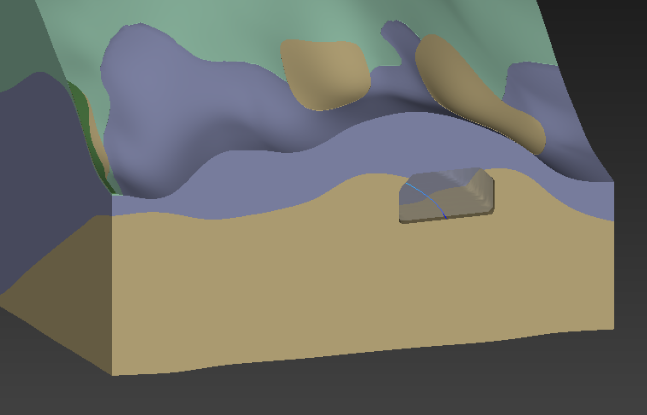
3d estimation - EFF file representing a uniform field: The file below is an abbreviated example of writing the output of 3d estimation having kriged a uniform field (which can be volume rendered). Large sections of the data regions of this file are omitted to save space. This is represented by sections of the file with “*** omitted ***” replacing many lines of data.

DEFINITION Mesh_Unif+Node_Data

NSPACE 3

NDIM 3

DIMS 41 41 35

COORD_UNITS “ft”

NUM_NODE_DATA 7

POINTS 11281.910004 12211.149994 -29.900000 12515.890015 13259.449951 0.900000

NODE_DATA_DEF 0 “VOC” “log_ppm” IN_FILE

NODE_DATA_DEF 1 “Confidence-VOC” “linear_%” IN_FILE

NODE_DATA_DEF 2 “Uncertainty-VOC” “linear_Unc” IN_FILE

NODE_DATA_DEF 3 “Geo_Layer” “linear_” IN_FILE

NODE_DATA_DEF 4 “Elevation” “linear_ft” IN_FILE

NODE_DATA_DEF 5 “Layer Thickness” “linear_ft” IN_FILE

NODE_DATA_DEF 6 “Material_ID” “linear_” IN_FILE

NODE_DATA_START

-2.357487 34.455845 2.325005 0.000000 -29.900000 30.799999 0.000000

-3.000000 34.977974 0.000000 0.000000 -29.900000 30.799999 0.000000

-3.000000 35.603794 0.000000 0.000000 -29.900000 30.799999 0.000000

***** OMITTED *****

-3.000000 30.056839 0.000000 0.000000 0.900000 30.799999 0.000000

-3.000000 29.858747 0.000000 0.000000 0.900000 30.799999 0.000000

-3.000000 29.673925 0.000000 0.000000 0.900000 30.799999 0.000000

END

3d estimation - EFF Split file representing a uniform field: The file below is a complete example of writing the output of 3d estimation having kriged a uniform field (which can be volume rendered). Note that the .EFF file is quite small, but references the data in a separate file named krig_3d_uniform_split.nd.

DEFINITION Mesh_Unif+Node_Data

NSPACE 3

NDIM 3

DIMS 41 41 35

COORD_UNITS “ft”

NUM_NODE_DATA 7

POINTS 11281.910004 12211.149994 -29.900000 12515.890015 13259.449951 0.900000

NODE_DATA_DEF 0 “VOC” “log_ppm” FILE “krig_3d_uniform_split.nd” ROW 1 COLS 1

NODE_DATA_DEF 1 “Confidence-VOC” “linear_%” FILE “krig_3d_uniform_split.nd” ROW 1 COLS 2

NODE_DATA_DEF 2 “Uncertainty-VOC” “linear_Unc” FILE “krig_3d_uniform_split.nd” ROW 1 COLS 3

NODE_DATA_DEF 3 “Geo_Layer” “linear_” FILE “krig_3d_uniform_split.nd” ROW 1 COLS 4

NODE_DATA_DEF 4 “Elevation” “linear_ft” FILE “krig_3d_uniform_split.nd” ROW 1 COLS 5

NODE_DATA_DEF 5 “Layer Thickness” “linear_ft” FILE “krig_3d_uniform_split.nd” ROW 1 COLS 6

NODE_DATA_DEF 6 “Material_ID” “linear_” FILE “krig_3d_uniform_split.nd” ROW 1 COLS 7

END

Large sections of the data regions of the data file krig_3d_uniform_split.nd are omitted below to save space. This is represented by sections of the file with “*** omitted ***” replacing many lines of data.

-2.357487 34.455845 2.325005 0.000000 -29.900000 30.799999 0.000000

-3.000000 34.977974 0.000000 0.000000 -29.900000 30.799999 0.000000

-3.000000 35.603794 0.000000 0.000000 -29.900000 30.799999 0.000000

***** OMITTED *****

-3.000000 30.056839 0.000000 0.000000 0.900000 30.799999 0.000000

-3.000000 29.858747 0.000000 0.000000 0.900000 30.799999 0.000000

-3.000000 29.673925 0.000000 0.000000 0.900000 30.799999 0.000000

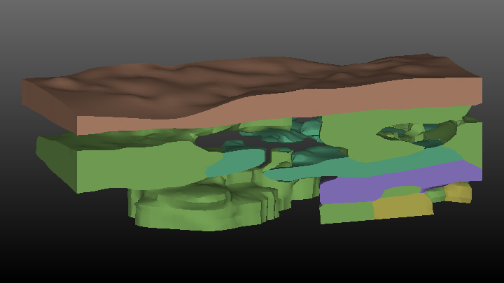
gridding and horizons & 3d estimation - EFF file representing multiple geologic layers with analyte (e.g. chemistry): The file below is an abbreviated example of writing the output of 3d estimation having kriged analyte (e.g. chemistry) data with geology input. Large sections of the data regions of this file are omitted to save space. This is represented by sections of the file with “*** omitted ***” replacing many lines of data.

NSPACE 3

NNODES 66355

COORD_UNITS “ft”

NUM_NODE_DATA 7

NCELL_SETS 5

NODES IN_FILE

11153.998856 12722.725708 2.970446

11161.871033 12715.198792 2.783408

11169.743210 12707.671875 2.594242

***** OMITTED *****

11250.848221 12865.266907 -42.575920

11248.750000 12870.909973 -42.000000

11243.389938 12870.020935 -42.474934

NODE_DATA_DEF 0 “TOTHC” “log_mg/kg” IN_FILE

NODE_DATA_DEF 1 “Confidence-TOTHC” “linear_%” IN_FILE

NODE_DATA_DEF 2 “Uncertainty-TOTHC” “linear_Unc” IN_FILE

NODE_DATA_DEF 3 “Geo_Layer” “Linear_” IN_FILE

NODE_DATA_DEF 4 “Elevation” “Linear_ft” IN_FILE

NODE_DATA_DEF 5 “Layer Thickness” “Linear_ft” IN_FILE

NODE_DATA_DEF 6 “Material_ID” “Linear_” IN_FILE

NODE_DATA_START

-0.777059 27.239126 15.861248 0.000000 2.970446 8.270601 2.000000

-0.661227 27.349216 16.503609 0.000000 2.783408 8.270658 2.000000

-0.288564 27.512394 18.822187 0.000000 2.594242 8.261375 2.000000

***** OMITTED *****

2.886921 69.551514 1.128253 4.000000 -42.575920 13.628321 4.000000

3.113943 99.999977 0.000000 4.000000 -42.000000 13.654032 4.000000

3.070153 72.869553 0.841437 4.000000 -42.474934 13.646055 4.000000

CELL_SET_DEF 0 8120 Hex “Fill” IN_FILE

CELL_SET_DEF 1 14680 Hex “Silt” IN_FILE

CELL_SET_DEF 2 6502 Hex “Clay” IN_FILE

CELL_SET_DEF 3 11284 Hex “Gravel” IN_FILE

CELL_SET_DEF 4 14412 Hex “Sand” IN_FILE

CELL_START

0 1 42 41 1681 1682 1723 1722

1 2 43 42 1682 1683 1724 1723

2 3 44 43 1683 1684 1725 1724

***** OMITTED *****

54462 54503 66349 66348 56143 56184 66353 66352

54503 54502 66350 66349 56184 56183 66354 66353

54502 54461 66347 66350 56183 56142 66351 66354

END

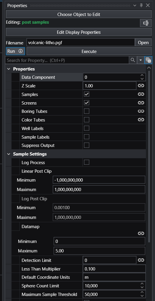
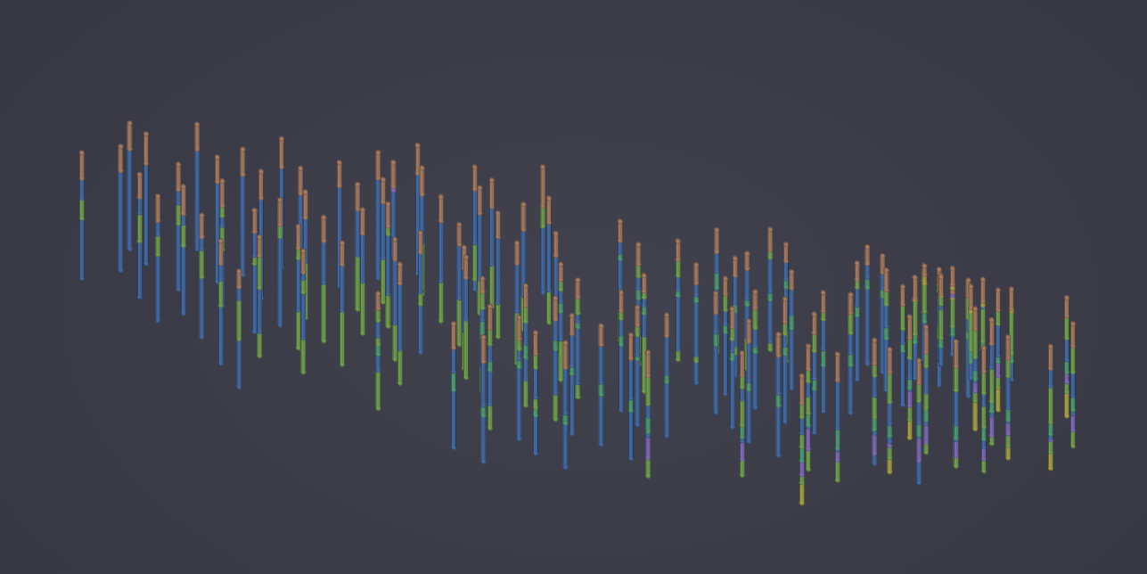
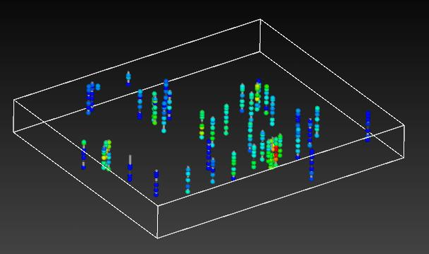
Post_samples - EFF file representing spheres: The file below is a complete example of writing the output of post_samples’ blue-black field port having read the file initial_soil_investigation_subsite.apdv. This data file has 99 samples with data that was log processed. If this file is read by read evs field. It creates all 99 spheres colored and sized as they were in Post_samples. The tubes and any labeling are not included in the field port from which this file was created.

DEFINITION Mesh+Node_Data

NSPACE 3

NNODES 99

COORD_UNITS “units”

NUM_NODE_DATA 2

NCELL_SETS 1

NODES IN_FILE

11566.340027 12850.590027 -10.000000

11566.340027 12850.590027 -70.000000

11566.340027 12850.590027 -160.000000

11586.340027 13050.589966 -10.000000

11586.340027 13050.589966 -70.000000

11586.340027 13050.589966 -160.000000

11381.700012 12747.500000 -15.000000

11381.700012 12747.500000 -25.000000

11414.399994 12781.099976 -15.000000

11414.399994 12781.099976 -25.000000

11338.000000 12830.799988 -10.000000

11338.000000 12830.799988 -65.000000

11338.000000 12830.799988 -115.000000

11338.000000 12830.799988 -165.000000

11410.290009 12724.690002 -5.000000

11410.290009 12724.690002 -35.000000

11410.290009 12724.690002 -45.000000

11410.290009 12724.690002 -125.000000

11410.290009 12724.690002 -175.000000

11427.000000 12780.900024 -10.000000

11427.000000 12780.900024 -30.000000

11427.000000 12780.900024 -80.000000

11416.899994 12819.450012 -10.000000

11416.899994 12819.450012 -30.000000

11416.899994 12819.450012 -70.000000

11416.899994 12819.450012 -95.000000

11416.899994 12819.450012 -105.000000

11416.899994 12819.450012 -120.000000

11416.899994 12819.450012 -140.000000

11401.730011 12897.770020 -10.000000

11401.730011 12897.770020 -30.000000

11401.730011 12897.770020 -80.000000

11401.730011 12897.770020 -110.000000

11401.730011 12897.770020 -145.000000

11401.730011 12897.770020 -180.000000

11259.670013 12819.289978 -10.000000

11259.670013 12819.289978 -40.000000

11259.670013 12819.289978 -70.000000

11259.670013 12819.289978 -95.000000

11259.670013 12819.289978 -140.000000

11340.489990 12892.609985 -30.000000

11340.489990 12892.609985 -55.000000

11340.489990 12892.609985 -80.000000

11340.489990 12892.609985 -110.000000

11340.489990 12892.609985 -130.000000

11340.489990 12892.609985 -165.000000

11248.750000 12870.909973 -10.000000

11248.750000 12870.909973 -35.000000

11248.750000 12870.909973 -45.000000

11248.750000 12870.909973 -85.000000

11248.750000 12870.909973 -110.000000

11248.750000 12870.909973 -160.000000

11248.750000 12870.909973 -210.000000

11086.519997 12830.669983 -15.000000

11086.519997 12830.669983 -30.000000

11086.519997 12830.669983 -80.000000

11086.519997 12830.669983 -130.000000

11211.869995 12710.750000 -30.000000

11211.869995 12710.750000 -80.000000

11211.869995 12710.750000 -135.000000

11199.039993 12810.159973 -20.000000

11199.039993 12810.159973 -40.000000

11199.039993 12810.159973 -85.000000

11199.039993 12810.159973 -150.000000

11298.000000 12808.630005 -60.000000

11496.339996 12753.590027 -10.000000

11496.339996 12753.590027 -30.000000

11496.339996 12753.590027 -80.000000

11496.339996 12753.590027 -110.000000

11496.339996 12753.590027 -150.000000

11309.029999 12948.989990 -10.000000

11309.029999 12948.989990 -35.000000

11309.029999 12948.989990 -95.000000

11309.029999 12948.989990 -125.000000

11309.029999 12948.989990 -130.000000

11209.350006 12993.940002 -5.000000

11209.350006 12993.940002 -35.000000

11209.350006 12993.940002 -60.000000

11209.350006 12993.940002 -95.000000

11209.350006 12993.940002 -125.000000

11301.970001 13079.660034 -20.000000

11301.970001 13079.660034 -30.000000

11301.970001 13079.660034 -85.000000

11301.970001 13079.660034 -125.000000

11286.769989 13026.699951 -30.000000

11286.769989 13026.699951 -45.000000

11286.769989 13026.699951 -75.000000

11286.769989 13026.699951 -120.000000

11393.470001 12948.900024 -20.000000

11393.470001 12948.900024 -45.000000

11393.470001 12948.900024 -95.000000

11393.470001 12948.900024 -110.000000

11393.470001 12948.900024 -130.000000

11393.470001 12948.900024 -170.000000

11251.300003 12929.270020 -10.000000

11251.300003 12929.270020 -30.000000

11251.300003 12929.270020 -80.000000

11251.300003 12929.270020 -120.000000

11251.300003 12929.270020 -145.000000

NODE_DATA_DEF 0 “TOTHC” “log_mg/kg” IN_FILE

NODE_DATA_DEF 1 "" "" ID 668 IN_FILE

NODE_DATA_START

-3.000000 4.998203

-3.000000 4.998203

-3.000000 4.998203

-3.000000 4.998203

-3.000000 4.998203

-3.000000 4.998203

-3.000000 4.998203

-3.000000 4.998203

-3.000000 4.998203

-3.000000 4.998203

1.322219 4.998203

2.806180 4.998203

1.602060 4.998203

-3.000000 4.998203

-3.000000 4.998203

-3.000000 4.998203

-3.000000 4.998203

-3.000000 4.998203

-3.000000 4.998203

1.845098 4.998203

2.278754 4.998203

-3.000000 4.998203

1.296665 4.998203

-3.000000 4.998203

1.278754 4.998203

3.716003 4.998203

1.623249 4.998203

1.505150 4.998203

-3.000000 4.998203

1.707570 4.998203

-3.000000 4.998203

3.770852 4.998203

3.869232 4.998203

1.113943 4.998203

-3.000000 4.998203

2.025306 4.998203

3.434569 4.998203

3.594039 4.998203

2.454845 4.998203

-3.000000 4.998203

2.740363 4.998203

2.079181 4.998203

3.806180 4.998203

4.908485 4.998203

2.176091 4.998203

-3.000000 4.998203

3.792392 4.998203

3.362897 4.998203

4.255272 4.998203

3.699387 4.998203

3.518514 4.998203

3.301030 4.998203

3.113943 4.998203

-3.000000 4.998203

-3.000000 4.998203

-3.000000 4.998203

-3.000000 4.998203

1.361728 4.998203

-3.000000 4.998203

-3.000000 4.998203

2.000000 4.998203

1.643453 4.998203

1.732394 4.998203

1.643453 4.998203

3.556303 4.998203

-0.522879 4.998203

-3.000000 4.998203

-3.000000 4.998203

-3.000000 4.998203

-3.000000 4.998203

3.079181 4.998203

-3.000000 4.998203

2.633468 4.998203

1.505150 4.998203

-3.000000 4.998203

-3.000000 4.998203

-0.920819 4.998203

-3.000000 4.998203

-3.000000 4.998203

-3.000000 4.998203

-0.886057 4.998203

-3.000000 4.998203

-3.000000 4.998203

-3.000000 4.998203

-3.000000 4.998203

-3.000000 4.998203

-0.096910 4.998203

-3.000000 4.998203

4.000000 4.998203

2.000000 4.998203

1.602060 4.998203

1.000000 4.998203

-0.301030 4.998203

-3.000000 4.998203

1.785330 4.998203

-3.000000 4.998203

0.431364 4.998203

4.518514 4.998203

-3.000000 4.998203

CELL_SET_DEF 0 99 Point "" IN_FILE

CELL_START

0

1

2

3

4

5

6

7

8

9

10

11

12

13

14

15

16

17

18

19

20

21

22

23

24

25

26

27

28

29

30

31

32

33

34

35

36

37

38

39

40

41

42

43

44

45

46

47

48

49

50

51

52

53

54

55

56

57

58

59

60

61

62

63

64

65

66

67

68

69

70

71

72

73

74

75

76

77

78

79

80

81

82

83

84

85

86

87

88

89

90

91

92

93

94

95

96

97

98

END

import vtk

import vtk reads a dataset from any of the following 9 VTK file formats. Please note that VTK’s file formats do not include coordinate units information, nor analyte units. There is a parameter which allows you to specify coordinate units (meters are the default).

  • vtk: legacy format
  • vtr: Rectilinear grids
  • vtp: Polygons (surfaces)
  • vts: Structured grids
  • vtu: Unstructured grids
  • pvtp: Partitioned Polygons (surfaces)
  • pvtr: Partitioned Rectilinear grids
  • pvts: Partitioned Structured grids
  • pvtu: Partitioned Unstructured grids

Ports

DirectionNameTypeDescription
OutputOutputFieldA field containing VTK file contents.
OutputOutput ObjectRenderableA renderable object displaying the VTK file contents.

Properties

PropertyTypeDescription
FilenameStringThe field file to read.
Use Application OriginBooleanWhen true, the module will apply the Application Origin. When false, data will be left in internal model space. Turn off when loading data intended to use as a glyph or similar.
ExecuteButtonThe Execute button forces the module to run.
UnitsStringThe coordinate units.

import cad

The import cad module will read the following versions of CAD files:

  • AutoCAD DWG and DXF files through AutoCAD 2021 (version 24.0)
  • Bentley Microstation DGN files through Version 8.

This module provides the user with the capability to integrate site plans, buildings, and other 2D or 3D features into the EVS visualization, to provide a frame of reference for understanding the three dimensional relationships between the site features, and characteristics of geologic, hydrologic, and chemical features. The drawing entities are treated as three dimensional objects, which provides the user with a lot of flexibility in the placement of CAD objects in relation to EVS objects in the visualization. The project onto surface and geologic_surfmap modules allow the user to drape CAD line-type entities (not 3D-Faces) onto three dimensional surfaces.

Virtually all AutoCAD object types are supported including points, lines (of all types), 3D surface objects and 3D volumetric objects.

AutoCAD drawings can be drawn in model space (MSPACE) or paper space (PSPACE). Drawings in paper space have a defined viewport which has coordinates near the origin. When read into EVS this creates objects which are far from your true model coordinates. For this reason, all drawings for use in our software should be in model space.

Ports

DirectionNameTypeDescription
InputInput Z ScaleNumberThe factor for vertical scaling.
OutputOutput Z ScaleNumberThe factor for vertical scaling.
OutputOutputFieldA field containing the CAD data.
OutputOutput ObjectRenderableA renderable object displaying the CAD data.

Properties

PropertyTypeDescription
FilenameStringThe name of the CAD dwg, dxf, or dgn file to be rendered.
Z ScaleDoubleThe Z Scale is the vertical exaggeration to be applied to the output object.
Use Application OriginBooleanWhen true, the module will apply the Application Origin. When false, data will be left in internal model space. Turn off when loading data intended to use as a glyph or similar.
ExecuteButtonThe Execute button forces the module to run.

Data Processing

PropertyTypeDescription
Render ModeChoice: Model Default, Wire-frame, Flat-ShadedThe Render Mode options allow you to choose how the CAD data will be rendered. Please read the module help for more details.
Unit HandlingChoice: Units From File, Force Default UnitsThe Unit Handling option determines whether we try to use units from the CAD file, or force the use of the default coordinate units.
Default Coordinate UnitsStringThe units to use when the units cannot be determined from the CAD file.
Remove Coincident NodesBooleanThe Remove Coincident Nodes toggle causes the reader to process the data, removing coincident nodes. This takes longer to process but creates a smaller more efficient representation of your CAD data.
Include Hidden LayersBooleanThe Include Hidden Layers toggle will cause CAD layers marked as hidden to be drawn.
Remove Points And Degenerate CellsBooleanThe Remove Point and Degenerate Cells option will remove all points and degenerate cells from the output.
Show As WireframeBooleanThe Show As Wire-frame toggle outlines surfaces. It is equivalent to setting Line Rendering to ‘regular’.
Color For WhiteColorThe Color For White button allows the user to set the color for any feature colored white.
Deviation For CurvesDoubleThe Deviation for Curves field allows the user to specify the accuracy with which analytical curves (arcs, circles) are displayed. The default value of 0.0 employs an expert system algorithm to determine a reasonable value based on the overall size of your CAD model.
Normal For 3D SolidsDoubleThe Normal for 3D Solids specifies the tolerance for parallel faces.
Separate LayersBooleanThe Separate Layers toggle causes each layer in the CAD file to be output as a separate cell set in EVS.
Layer DetailsMulti-selectThe Data To Include allows the user to set which sets of data to render.
Remove Empty 0 LayerBooleanWhether to remove a layer named ‘0’ that draws nothing, or not. This is primarily intended for removing AutoCAD’s default layer when it contains no visible objects.

import vector gis

The import vector gis module reads the following vector file formats: ESRI Shapefile (*.shp); Arc/Info E00 (ASCII) Coverage (*.e00); Atlas BNA file (*.bna); GeoConcept text export (*.gxt); GMT ASCII Vectors (*.gmt); and the MapInfo TAB (*.tab) format.

Ports

DirectionNameTypeDescription
InputInput Z ScaleNumberThe factor for vertical scaling.
OutputOutput Z ScaleNumberThe factor for vertical scaling.
OutputOutputFieldA field containing the vector GIS data.
OutputOutput ObjectRenderableA renderable object displaying the vector GIS data.

Properties

PropertyTypeDescription
FilenameStringThe name of the Vector file format to read.
Z ScaleDoubleThe Z Scale is the vertical exaggeration to apply to the input data.
Use Application OriginBooleanWhen true, the module will apply the Application Origin. When false, data will be left in internal model space.
ExecuteButtonThe Execute button forces the module to run.

Data Processing

PropertyTypeDescription
Coordinate UnitsStringThe Coordinate Units string allows the user to specify the units for the coordinates in the input data. Defaults to the units in the spatial reference of the input vector file, if available. Otherwise, default of meters (m) is assumed.
Assign Data To ZBooleanIf the Assign Data To Z toggle is on and Include Attributes As Data is on, then the selected data will be assigned as the Z coordinate.
Data To Assign To ZChoiceThe Data To Assign To Z choice allows the user to select which data is assigned as the z coordinates.
Data To OutputMulti-selectThe Data to Output choice allows the user to select the cell data to include in the output.

import raster as horizon

The import raster as horizon module reads several different raster format files in EVS Geology format. These formats include DEMs, Surfer grid files, Mr. Sid files, ADF files, etc.. Multiple import raster as horizon modules can be combined with combine horizons into a 3D geologic model. Alternatively, a single file can be displayed as a surface (with surfaces from horizons) or you can export its coordinates (with export nodes) to use the values in a GMF file.

Ports

DirectionNameTypeDescription
OutputOutput Geologic FieldFieldThe main geologic field output from the module.
OutputGeology Export OutputVistas DataInformation required for direct exporting of geology to other software.
OutputGeologic Legend InformationGeology LegendInformation required to properly label stratigraphic output or lithology within Legend.

Properties

PropertyTypeDescription
Allow RunBooleanThe Allow Run toggle if selected will allow the module to run when any of the input parameters are changed. If the toggle is not selected then the Execute button will have to be pressed for the module to run.
ExecuteButtonThe Execute button forces the module to run. If this has been pressed and the application saved, it will cause the module to run when the application is loaded.
FilenameStringThe raster_to_geology module reads several different raster format files in EVS Geology format. These formats include DEMs, Surfer grid files, Mr. Sid files, ADF files, etc..
Material NumberIntegerThe Material Number type in allows the user to set the material number for the surface being read.
Coord UnitsStringThe Coord Units type in allows the user to set the coordinate units for the surface being read.
Surface NameStringThe Surface Name type in allows the user to set the surface name for the surface being read.

Surface Controls

PropertyTypeDescription
Raster BandIntegerThe Raster Band is used to select a single raster band when reading image formats such as jpeg or tif.
DownsizeIntegerThe Downsize value is used to reduce the resolution of the input raster.
Blanks As NullBooleanThe Blanks as Null option is used to specify that points marked to be blanked out in the raster will be left out of the geologic model when it is created. It is highly recommended to leave this checked.
Min IIntegerThe Min I value is used to crop the lower bound of the horizontal domain of the raster.
Max IIntegerThe Max I value is used to crop the upper bound of the horizontal domain of the raster.
Min JIntegerThe Min J value is used to crop the lower bound of the vertical range of the raster.
Max JIntegerThe Max J value is used to crop the upper bound of the vertical range of the raster.
Max Total ResolutionIntegerThe Max Total Resolution will cause the module to report an error if the generated geology is greater than the set amount.

buildings

The buildings module reads C Tech’s .BLDG file and creates various 3D objects (boxes, cylinders, wedge-shapes for roofs, simple houses etc.), and provides a means for scaling the objects and/or placing the objects at user specified locations. The objects are displayed based on x, y & z coordinates supplied by the user in a .bldg file, with additional scaling option controls on the buildings user interface.

Each object is made up of 3D volumetric elements. This allows for the output of buildings to be cut or sliced to reveal a cross section through the buildings.

Ports

DirectionNameTypeDescription
InputInput Z ScaleNumberThe factor for vertical scaling.
OutputOutput Z ScaleNumberThe factor for vertical scaling.
OutputOutputFieldA field containing the buildings.
OutputOutput ObjectRenderableA renderable object displaying the buildings.

Properties

PropertyTypeDescription
Import FileStringImport an existing *.bldg file.
Reload Import FileButtonThe Reload Import File will force the module to load the import file and run.
Z ScaleDoubleZ Scale is required to assure that buildings are matched to scaled input.
Building Height ScaleDoubleThe Building Height Scale will vertically exaggerate the height of each building.
Building OffsetDoubleThe Building Offset will move all buildings vertically by the set amount.
Export FileStringExport current buildings to a *.bldg file.

Default Building Settings

PropertyTypeDescription
Default NameStringThe default name for each new building added.
Increment Building IdBooleanNew buildings will have an Identifier greater that the value of the last building on the list.
Default OffsetDoubleThe vertical offset for each new building.
Default HeightDoubleThe height to set for each new building.
Default WidthDoubleThe width to set for each new building.
Default LengthDoubleThe length to set for each new building.
Default AzimuthDoubleThe azimuth to align each new building to.
Default TypeChoice: Box (0), Roof Gable (1), Wedge (2), Triangle (3), Right Triangle (4), 6 Sided Cylinder (5), 8 Sided Cylinder (6), 16 Sided Cylinder (7), 32 Sided Cylinder (8), 16 Sided Tank (9), 32 Sided Tank (10), Roof Corner 1 (11), Roof Corner 2 (12), Roof Corner 3 (13), Cone (14), 1 Story Building (15), 2 Story Building (16), 1 Story House (17), 2 Story House (18)The type for each new building.
Default IdIntegerThe Identifier for each new building.
Default ColorColorThe color for new buildings.

Building Settings

PropertyTypeDescription
Probe ActionChoice: None, Reset Position, Add BuildingAllows for the changing of the building center or for adding a new building at the probed location. Only available when the viewer is connected.
Outline Current BuildingBooleanThe Outline Current Building turns on or off a bounding rectangle showing the current building being edited.
Delete Current BuildingButtonThis command will remove the currently selected building from the list of buildings.
Current BuildingChoiceThe Current Building allows the user to select a single building to edit.
Current Building ValuesBuildingThe Current Building Values.
  • Sample Buildings File

    Sample Buildings File Below is an example buildings file. Note that the last 4 columns are optional and contain RGB color values (three numbers from zero to 1.0) and/or a building ID number that can be used for coloring. If only color values are supplied (3 numbers) the ID is automatically determined by the row number. If four numbers are provided it is assumed that the last one is the ID. If only one number is provided it is the ID.

Subsections of buildings

Sample Buildings File

Below is an example buildings file. Note that the last 4 columns are optional and contain RGB color values (three numbers from zero to 1.0) and/or a building ID number that can be used for coloring. If only color values are supplied (3 numbers) the ID is automatically determined by the row number. If four numbers are provided it is assumed that the last one is the ID. If only one number is provided it is the ID.

The file below is shown in a table (with dividing lines) for clarity only. The first uncommented line is the number 16 which defines the number of rows of buildings data. The actual file is a simple ASCII file with separators of space, comma and/or tab.

EVS

Copyright (c) 1994-2008 by

C Tech Development Corporation

All Rights Reserved

# This software comprises unpublished confidential information of

# C Tech Development Corporation and may not be used, copied or made

# available to anyone, except in accordance with the license

# under which it is furnished.

C Tech 3D Building file

Building 0 is a unit box with base at z=0.0 centered at origin x,y

Building 1 is a gabled roof for the unit box

# (to make it a house) with base at z=0.0 centered at origin x,y

Building 2 is a wedge roof for the unit box

# (to make it a house) with base at z=0.0 centered at origin x,y

Building 3 is a Equilateral (or Isoseles) Triangular Building 3 side

Building 4 is a Right Triangular Building 3 side

Building 5 is a Hexagonal (6 side) cylinder

Building 6 is a Octagonal (8 side) cylinder

Building 7 is a 16 side cylinder

Building 8 is a 32 side cylinder

Building 9 is a 16 sided horiz. cylindrical tank (Height & Width equal diameter, Length is along x)

Building 10 is a 32 sided horiz. cylindrical tank (Height & Width equal diameter, Length is along x)

Building 11 is a right angle triangle, height only at right angle

Building 12 is a right angle triangle, height at non-right angle

Building 13 is a right angle triangle, height at right angle and 1 non-right angle

Lines beginning with “#” are comments

First uncommented line is number of buildings

X Y Z LengthWidthHeight Angle Bldg_Type Color and/orID

16

0010505020001
010005050303002
0100306050203012
020005050301003
0200305050251023
20000505050034
10010004040201545
20010004040303056
2002000505050067
1002000406020-4578
10000505040089
30000602020-4590.80.60.410
30010005050300100.40.60.411
030005050500111.00.40.412
10030005050500120.41.00.413
20030005050500130.40.41.014

read lines

The read lines module is used to visualize a series of points with data connected by lines. read lines accepts three different file formats, with the APDV file format the lines are connected by boring ID, with the ELF (EVS Line File) format each line is made by defining the points that make up the line, and with the SAD (Strike and Dip) file format, there is a choice to connect each sample by ID or by Data Value.

SAD files connect by ID – If a *.sad file has been read the lines will be connected by ID.

SAD files connect by Data – If a *.sad file has been read the lines will be connected by the data component.

Ports

DirectionNameTypeDescription
InputInput Z ScaleNumberThe factor for vertical scaling.
OutputOutput Z ScaleNumberThe factor for vertical scaling.
OutputOutput FieldFieldA field containing the line model.
OutputOutput ObjectRenderableA renderable object displaying the line model.

Properties

PropertyTypeDescription
FilenameStringThe filename to process into lines. EVS Line Files (elf), Strike and Dip Files (sad), or Analytical Point Data Values (apdv) can be used as input.
ExecuteButtonThe Execute button forces the module to run.
Z ScaleDoubleThe vertical exaggeration of the output lines.
Data ComponentIntegerThis Data Component controls which data value to color the lines by.
Use Application OriginBooleanWhen true, the module will apply the Application Origin. When false, data will be left in internal model space. Turn off when loading cross section paths or similar.

Data Processing

PropertyTypeDescription
Log Process Nodal DataBooleanThis toggle sets the nodal data values to the log value of the input node data.
Log Process Cell DataBooleanThis toggle sets the cell data values to the log value of the input cell data.
Connectivity ComponentChoice: SAD file lines connected by ID, SAD file lines connected by DataThe Connectivity Component determines how SAD files are connected.
Clip MinDoubleThis is only active if either Log processing for nodal or cell data is selected and sets the minimum value for each data value so that they can be correctly processed.

Glyph Settings

PropertyTypeDescription
Create GlyphsBooleanThe Create Glyphs control will allow for the creation of user selected glyphs at each node in the input file.
Generated GlyphChoice: Sphere, Cube, Cone, Cylinder, Polygon, DiskThe Generated Glyph choice allows the user to select the type of glyph that is automatically generated.
Glyph SizeDoubleThe Glyph Size value is used to scale the glyphs in all directions. The default is automatically computed based on your input data.
Sphere SubdivisionsIntegerThe number of subdivisions to use for spheres. Larger numbers create more detailed sphere representations.
Glyph ResolutionIntegerThe resolution for generated cone, polygon, cylinder, and disk glyphs.
Primary Axis FactorDoubleThe scale factor for the primary axis of the glyph.
Secondary Axis FactorDoubleThe scale factor for the secondary axis of the glyph.
Heading DipDoubleThe Heading and Dip values are used to align the glyphs to a constant orientation.
RollDoubleThe roll of the glyph along its primary axis.
Include Center DataBooleanThe Include Center Data toggle will tell the module to include the center point of each glyph as a cell data component. This allows the user to probe onto the glyph and return its center instead of the position on the outside of the glyph.

EVS Line File Example

Discussion of EVS Line Files

EVS line files contain horizontal and vertical coordinates, which describe the 3-D locations and values of properties of a system. Line files must be in ASCII format and can be delimited by commas, spaces, or tabs. They must have an .elf suffix to be selected in the file browsers of EVS modules. Each line of the EVS line file contain the coordinate data for one sampling location and up to 300 (columns of) property values. There are no computational restrictions on the number of lines that can be included in a file.

EVS Line Files

EVS Line Files consist of file tags that delineate the various sections of the file(s) and data (coordinates, nodal and/or cell data). The file tags are discussed below followed by portions of a few example files.

FILE TAGS:

The file tags for the ASCII file formats (shown in Bold Italics) are discussed below with a representative example. They are given in the appropriate order. If you need assistance creating software to write these file formats, please contact support@ctech.com.

COORD_UNITS “ft” Defines the coordinate units for the file. These should be consistent in X, Y, and Z.

NUM__DATA 7 1

Number of nodal data components followed by the number of cell data components.

NODE_DATA_DEF 0 “TOTHC” “log_ppm”

NODE_DATA_DEF specifies the definition of a nodal data component. The second value is the data component number, the third is the name, and the 4th is the units.

CELL_DATA_DEF 0 “Indicator” “Discreet Unit”

Definition of cell data. Same options as NODE_DATA_DEF

LINE 12 1

Beginning of a line segment is followed on the same line by the cell data values.

Following this line should be the points making up the line in the following format:

X, Y, Z coordinates followed by nodal data values.

64718.310547 37500.000000 -1250.000000 1 -1250.000000

63447.014587 35101.682129 -2000.000000 2 -2000.000000

CLOSED

This flag is used at the end of a line definition to indicate the end of the line should be connected to the beginning of the line.

END

Marks the end of the data section of the file. (Allows us to put a password on .eff files)

EXAMPLE FILE

NUM_DATA 2 0

NODE_DATA_DEF 0 “Node_Number” “Linear_ID”

NODE_DATA_DEF 1 “Distance” “Linear_ft”

LINE

1900297.026154 677367.319824 72.000000 0.000000 0.000000

1900314.256775 677438.611328 72.000000 1.000000 73.344208

1900314.687561 677442.703522 72.000000 2.000000 77.459015

1900316.410645 677447.011261 72.000000 3.000000 82.098587

1900319.641266 677447.442018 72.000000 4.000000 85.357796

1900345.487030 677441.411530 72.000000 5.000000 111.897774

1900360.563782 677439.472870 72.000000 6.000000 127.098656

1900363.579193 677447.226807 72.000000 7.000000 135.418289

1900365.517822 677447.226807 72.000000 8.000000 137.356918

1900365.948608 677438.396118 72.000000 9.000000 146.198105

1900379.733032 677436.888245 72.000000 10.000000 160.064758

1900405.578766 677432.150055 72.000000 11.000000 186.341217

1900497.331879 677416.427002 72.000000 12.000000 279.431763

1900511.331512 677414.919464 72.000000 13.000000 293.512329

1900525.762268 677411.257721 72.000000 14.000000 308.400421

1900527.269775 677405.442444 72.000000 15.000000 314.407898

1900524.900696 677399.411926 72.000000 16.000000 320.887085

1900522.531311 677391.012024 72.000000 17.000000 329.614746

1900517.362366 677357.196808 72.000000 18.000000 363.822754

1900501.854828 677266.951569 72.000000 19.000000 455.390686

1900501.639282 677262.213379 72.000000 20.000000 460.133789

1900500.777710 677255.321014 72.000000 21.000000 467.079773

1900496.470306 677250.151733 72.000000 22.000000 473.808472

1900487.208862 677241.751816 72.000000 23.000000 486.311798

1900450.378204 677201.906097 72.000000 24.000000 540.572083

1900403.568481 677152.368134 72.000000 25.000000 608.727478

1900356.758759 677102.830177 72.000000 26.000000 676.882874

1900309.949036 677053.292221 72.000000 27.000000 745.038269

1900286.257172 677028.523243 72.000000 28.000000 779.313721

1900278.718445 677022.923517 72.000000 29.000000 788.704651

1900269.672546 677024.431061 72.000000 30.000000 797.875305

1900217.334717 677035.200397 72.000000 31.000000 851.309631

1900232.196075 677097.230453 72.000000 32.000000 915.095154

1900247.057434 677159.260513 72.000000 33.000000 978.880615

1900252.226715 677179.937317 72.000000 34.000000 1000.193787

1900267.159851 677242.326401 72.000000 35.000000 1064.345215

1900282.093018 677304.715485 72.000000 36.000000 1128.496460

1900297.026154 677367.104584 72.000000 37.000000 1192.647827

END

read strike and dip

The read strike and dip module is used to visualize sampled locations. It places a disk, oriented by strike and dip, at each sample location. Each disk is probable and can be colored by a picked color, by Id, or by data value. If an ID is present, such as a boring ID, then there is an option to place tubes between connected disks, or those disks with similar Id’s.

Strike and dip refer to the orientation of a geologic feature. The strike is a line representing the intersection of that feature with the horizontal plane (though this is often the ground surface). Strike is represented with a line segment parallel to the strike line. Strike can be given as a compass direction (a single three digit number representing the azimuth) or basic compass heading (e.g. N, E, NW).

The dip gives the angle of descent of a feature relative to a horizontal plane, and is given by the number (0-90) as well as a letter (N,S,E,W, NE, SW, etc.) corresponding to the rough direction in which feature bed is dipping.

Info

We do not support the Right-Hand Rule, therefore all dip directions must have the direction letter(s).

Ports

DirectionNameTypeDescription
InputInput Z ScaleNumberThe factor for vertical scaling.
OutputOutput Z ScaleNumberThe factor for vertical scaling.
OutputOutputFieldA field containing the strike and dip model.
OutputOutput ObjectRenderableA renderable object displaying the strike and dip model.

Properties

PropertyTypeDescription
FilenameStringThe Filename of the Strike And Dip file (*.sad).
ExecuteButtonThe Execute button forces the module to run.
Z ScaleDoubleThe Z Scale is the vertical exaggeration to apply to the output.

Display Settings

PropertyTypeDescription
Disk Thickness PercentageDoubleThe Disk Thickness Percentage sets the thickness of each disk to a factor of the coordinate extents of the model.
Minimum Disk RadiusDoubleThis sets the minimum radius for each disk. The coordinates are in model coordinates.
Radius ExtentDoubleThe disk radius is based upon a percentage of the x, y, and z extents of the model.
Disk ResolutionIntegerNumber of prisms used to make each disk. The greater the number of prisms the more “round” the disk. Resolutions based on a factor of four are recommended as they will allow the dip and strike lines to end at the extents of the disk.
Include Dip As DataBooleanThis allows you to color the Dip lines based upon the dip angle.
Display Dip LinesBooleanThis toggle turns the Dip lines on and off.
Include Strike As DataBooleanThis allows you to color the Strike lines based upon the strike.
Display Strike LinesBooleanThis toggle turns the Strike lines on and off.
Connectivity ComponentChoice: SAD file lines connected by ID, SAD file lines connected by Data, Do not connect disks with linesThe Connectivity Component determines how SAD files are connected.
Display AsChoice: None, Tubes, WiresUse Display As to change how the boring lines are displayed, you can either turn off them off entirely, display them as tubes, or display them as wires.
Tube RadiusDoubleThis is the radius for the tubes, set by default to be 50 percent of the disk Radius Extent.
Tube ResolutionIntegerThis alters the number of sides each tube has, the more sides the more “round” the tubes will look, and possibly the slower they will display.
Main ColorColorEach boring tube is divided using two colors, the Main Color sets the first of these.
Secondary ColorColorEach boring tube is divided using two colors, the Secondary Color sets the second of these.
Color SeparationDoubleThe Color Separation defines the length both the Main Color and the Secondary Color will go to before switching to the other. This can be used as a visual clue as to the vertical scale of the model.
Include Center DataBooleanThe Include Center Data toggle will tell the module to include the center point of each tube end point as a cell data component. This allows the user to probe onto the tube and return its center instead of the position on the outside of the tube.

Strike and Dip File Example

Discussion of Strike and Dip Files

Strike and dip files consist of 3D coordinates along with two orientation values called strike and dip. A simple disk is placed at the coordinate location and then the disk is rotated about Z to match the strike and then rotated about Y to match the dip. An optional id and data value can be used to color the disk.

Format:

You may insert comment lines in C Tech Strike and Dip (.sad) input files. Comments can be inserted anywhere in a file and must begin with a ‘#’ character.

Strike can be defined in the following ways :

  1. For strikes running along an axis:

N, S, NS, SN are all equivalent to 0 or 180, and will always have a dip to E or W

E, W, EW, WE are all equivalent to 90 or 270, and will always have a dip to N or S

NE, SW are both equivalent to 135 or 315, and can have a dip specified to N, S, E, or W

NW, SE are both equivalent to 45 or 225, and can have a dip specified to N, S, E, or W

  1. For all other strikes: any compass direction between 0 and 360 degrees can be specified, with the dip direction clarifying which side of the strike is downhill.

Dip can be defined only in degrees in the range of 0 to 90.0 followed by a direction such as 35.45E

There is no required header for this file type.

Each line of the file must contain:

X, Y, Z, Strike, Dip, ID (optional), and Data (optional).

NOTE: The ID can only contain spaces if enclosed in quotation marks (ex “ID 1”).

EXAMPLE FILE

x y z strike dip

51.967 10.948 26.127 35.205 59.8031E

50.373 33.938 26.127 13.048 68.49984E

51.654 60.213 26.127 139.18 76.74215E

50.529 83.203 26.127 213.50 62.94599E

64.358 76.634 11.471 114.23 80.38694E

66.430 33.938 -6.849 41.421 60.38837E

75.901 50.360 -21.505 60.141 72.88960E

72.943 7.663 -21.505 5.255 65.51247E

101.90 30.654 -72.801 77.675 65.9524E

81.339 50.360 -43.489 244.95 70.7079E

72.263 73.350 -21.505 82.929 69.3159E

89.897 73.350 -61.809 31.531 55.6570E

END

FILE TAGS:

The file tags for the ASCII file formats (shown in Bold Italics) are discussed below with a representative example. They are given in the appropriate order. If you need assistance creating software to write these file formats, please contact support@ctech.com.

COORD_UNITS “ft” Defines the coordinate units for the file. These should be consistent in X, Y, and Z.

END (this is optional, but should be used if any lines will follow your actual data lines)

read glyph

read glyph replaces the Glyphs sub-library that was in the tools library. It reads glyphs saved in any of the three primary EVS field file formats and allows you to modify the shape and orientation of the glyph to allow it to be used in various modules that employ glyphs in slightly different ways. These include glyphs at nodes, place_glyph, drive_glyphs, advector, post_samples, etc. Most modules EXCEPT post_samples will use the glyphs without changing the default alignment. The supported file formats are:

  1. .eff ASCII format, best if you want to be able to open the file in an editor or print it

  2. .efz GNU Zip compressed ASCII, same as .eff but in a zip archive

  3. .efb binary compressed format, the smallest & fastest format due to its binary form

For a description of the .EFF file formats click here.

The objects saved in the .efx files should be simple geometric objects ideally designed to fit in a unit box centered at the origin (0,0,0). For optimal performance the objects should not include nodal or cell data. You may create your own objects or use any of the ones that C Tech supplies in the ctech\data\glyphs folder.

Ports

DirectionNameTypeDescription
OutputOutputFieldA field containing the glyph.
OutputOutput ObjectRenderableA renderable object displaying the glyph.

Properties

PropertyTypeDescription
FilenameStringThe field file containing the glyph object.
ExecuteButtonThe Execute button forces the module to run.
Offset BaseBooleanOffset Base is a toggle that changes the origin from the centroid of the glyph to the base.
AlignmentChoice: Orient For Vector, Align VerticallyThe Alignment allows the user to choose how to determine the orientation of the glyph.
RollDoubleThe Roll is a value that lets you control the rotation about the roll axis (glyph directional axis).
Length FactorDoubleLength Factor is a value that lets you scale the length of the glyph.
Width FactorDoubleWidth Factor is a value that lets you scale the width of the glyph.
Height FactorDoubleHeight Factor is a value that lets you scale the height of the glyph.

import geometry

The import geometry module will read STL, PLY, OBJ and .G files containing object geometries.

This module provides the user with the capability to integrate site plans, topography, buildings, and other 3D features into the EVS visualizations.

Info

This module intentionally does not have a Z-Scale port since this class of files are so often not in a user’s model projected coordinate system. Instead a Transform Settings group is provided that allows for a much more complex set of transformations including scaling, translations and rotations.

Ports

DirectionNameTypeDescription
OutputOutput FieldFieldThe main output field of the triangulated model.
OutputOutput ObjectRenderableA renderable object displaying the triangulated model.

Properties

PropertyTypeDescription
Allow RunBooleanThis toggle will prevent the module from running when turned to the Off position.
FilenameStringThe file containing the triangulated geometry.
ExecuteButtonThis button will allow the module to run one time even if the Allow Run toggle is turned to the off position. This allows the user to make multiple changes with only one update.
Use Application OriginBooleanWhen true, the module will apply the Application Origin. When false, coordinates will be left in internal model space.

Transform Settings

PropertyTypeDescription
Transform ListTransform FieldsThe list of transformations applied to the input field. This allows you to add any number of Translation, Scale, or Rotation transformations in order to place your geometry in the same coordinate space as the rest of your model.
  • write evs field

    Creates a file in one of 5 different formats containing all the mesh and nodal and/or cell data component information sent to the input port.

  • export web scene

    Export EVS scenes with vector output of 3D models for the C Tech Web Viewer.

  • export pdf scene

    Export EVS scenes with vector output of 3D models for the C Tech PDF Converter.

  • export 3d scene

    Export EVS scenes with vector output of 3D models for third party software usage.

  • export nodes

    Export an ASCII file containing the coordinates and optionally the data of any field in EVS.

  • export cad

    Write vector output of graphical results in industry standard AutoCAD DWG or DXF format or Microstation DGN format.

  • export surface to raster

    Create a file in one of the GeoTiff raster format.

  • export vector gis

    Create a file in one of the following vector formats: ESRI Shapefile (.shp); GMT ASCII Vectors (.gmt); and MapInfo TAB (*.tab).

  • export horizon to raster

    Create a raster file based on a single input horizon.

  • write lines

    Save a series of points with data connected by lines. These lines are stored in the EVS Line File format.

  • export horizons to vistas

    Write the fundamental geologic grid and horizon information to a file format that Ground Water Vistas can read.

Subsections of Export

write evs field

The write evs field module creates a file in one of several formats containing the mesh and nodal and/or cell data component information sent to the input port.

This module is useful for writing the output of modules which manipulate or interpolate data (3d estimation, 2d estimation, etc.) so that the data will not need to be processed in the future.

The saved and processed data can be read using read evs field, which is much faster than reprocessing the data.

Principal recommended format: EF2

  • The newest and strongly recommended format is EF2. This format is capable of containing additional field data and mesh types which are not supported in the legacy format. This is the only LOSSLESS format for current and future EVS fields. Although the files created in EF2 format are generally larger than EFBs, the further subsetting and/or processing of these updated fields can be dramatically more efficient.

    • Uniform fields
    • Geology (from gridding and horizons)
    • Structured fields (such as irregular fields read in from read evs field)
    • Unstructured Cell Data (UCD format) general grids with nodal and/or cell data
    • Special fields containing spheres (which are points with radii)
    • Special fields containing color data (such as LIDAR data)

Legacy formats:

  • The legacy formats below were the recommended formats in software releases before 2024. With enhancements to EVS Fields, these formats must be considered LOSSY, meaning that some data and the (EF2) optimized grids will be compromised if these formats are used. We strongly recommend using the EF2 format.
    • .eff ASCII format, best if you want to be able to open the file in an editor or print it. For a description of the EFF file formats click here.
    • .efz GNU Zip compressed ASCII, same as .eff but in a zip archive
    • .efb binary compressed format, the smallest and fastest format due to its binary form

Ports

DirectionNameTypeDescription
InputInput FieldFieldA field containing model to write to the EVS field file format.
InputGeologic Legend InformationGeology LegendInformation required to properly label stratigraphic output or lithology within Legend.
InputString 1StringA string to use as a variable.
InputFile NotesStringText containing the notes to be stored in the file.

Properties

PropertyTypeDescription
FilenameStringThe output filename. Saves datasets in EVS/MVS compatible file formats (EF2, EFB, EFZ, EFF).
Check For Cell Set DataBooleanCauses any cell data that is constant throughout its cell set to be written as a cell set data component.
Translate By OriginBooleanCauses the output to be written in the user’s coordinate space. When turned off, the output will be written around the origin.

Additional Information

PropertyTypeDescription
NotesStringNotes to include within the file. These are just comments and have no effect on the module.
DescriptionStringAllows the user to set the description in the output file.
AuthorStringAllows the user to set the author name on the output file.
OrganizationStringAllows the user to set the organization name on the output file.
ProjectStringAllows the user to set the project displayed in the output file.
StatusStringAllows the user to set the status displayed in the output file.
RestrictionsStringAllows the user to set the restrictions displayed in the output file.

Variables

PropertyTypeDescription
S1StringA string value that can be used as the variable {S1} in the expression.

Legacy File Options

PropertyTypeDescription
Split Into Separate FilesBoolean(Only applies to EFB/EFF/EFZ) Splits the output into separate files. The corresponding EFF or EFZ file will only contain the tag information. Any required nodes, data, or connectivity will be written into separate files.
Force Nodal Data In OutputBoolean(Only applies to EFB/EFF/EFZ) Causes the field definition to always contain Node_Data. If this is off and there are no node data components, a simpler Mesh-Only style field will be saved. This causes a mesh to save as a Mesh+Node_Data (with 0 data components), which will allow many modules to work with this data.
Force Cell Data In OutputBoolean(Only applies to EFB/EFF/EFZ) Same as above, but with cell data. Very few modules require cell data, so this is not on by default, but is provided as an option.

export web scene

The export web scene module connects via the view port and writes all objects in your view as a C Tech Web Scene (*.ctws), a single file which you and your customers can load and view at the C Tech web viewer.

Details on its use at How to Create C Tech Web Scenes.

WARNINGS:

  • DATAMAPS ARE USED FOR PROBING: When using unlinked values (Min and Max) such that the resulting datamap is a subset of the true data range, probing in C Tech Web Scenes will only be able to report values within the truncated data range. Values outside that limited range will display the nearest value within the truncated range. This applies to the use of the Datamap parameters in post samples or when the data range is truncated by clipping in the estimation modules or with the change min max module.

Ports

DirectionNameTypeDescription
InputViewViewThe view containing all associated renderable objects.
InputString 1StringA string to use as a variable.
InputZ ScaleNumberThe factor for vertical scaling.

Properties

PropertyTypeDescription
FilenameStringThe name of the output CTWS file to generate.
Favorite BookmarksBooleanFavorite Bookmarks in the resulting Web Scene.
Favorite Preset ViewsBooleanFavorite Preset Views in the resulting Web Scene.
Z ScaleDoubleThe vertical exaggeration applied to the input field. This scale will be used to remove all vertical exaggeration prior to writing.
Compress OutputBooleanTurning Compress Output off disables compression for the entire CTWS scene. If on, compression for individual modules can still be selectively excluded via red port options.
Include Preview ImageBooleanWhen selected, a preview image is written into the CTWS file for easier display while file browsing in Windows Explorer and EVS.
Full Size Preview ImageBooleanWhen selected and Include Preview Image is selected, the image will be saved at the resolution of the viewer. Otherwise a smaller default resolution will be used.
Run SequencesBooleanWhen selected, sequences will be run during the export process and their individual output will be included in the CTWS file. If not selected, only the current sequence state will be exported as a group object.
Restore Application Sequence StatesBooleanWhen selected, sequences will be restored to their initial state. This can save runtime if you don’t need a specific sequence state to be active. Otherwise, sequences will be left in their last state.

Scene Information

PropertyTypeDescription
DescriptionStringAllows the user to set the description in the output scene.
AuthorStringAllows the user to set the author name on the output scene.
OrganizationStringAllows the user to set the organization name on the output scene.
ProjectStringAllows the user to set the project displayed in the output scene.
StatusStringAllows the user to set the status displayed in the output scene.
RestrictionsStringAllows the user to set the restrictions displayed in the output scene.

Variables

PropertyTypeDescription
S1StringA string value that can be used as the variable {S1} in the expression.

Export Stage Script

PropertyTypeDescription
Script FilenameStringThe script called during the different stages of the export. This is intended to use with evs.get_export_stage() to allow operations to occur during the export process.

export pdf scene

The export pdf scene module connects via the view port and writes all objects in your view as a .evspdf file that C Tech’s PDF Converter can convert to a 3D PDF. This module requires a valid PDF Converter license in order to function.

Ports

DirectionNameTypeDescription
InputViewViewThe view containing all associated renderable objects.
InputZ ScaleNumberThe factor for vertical scaling.

Properties

PropertyTypeDescription
FilenameStringThe name of the output EVS PDF scene file to generate.
Z ScaleDoubleThe vertical exaggeration applied to the input field. This scale will be used to remove all vertical exaggeration prior to writing.
Compress OutputBooleanTurning Compress Output off disables compression for the entire scene. If on, compression for individual modules can still be selectively excluded via red port options.

export 3d scene

The export 3d scene module will export the entire view (model) in the following formats to allow importing to other 3D modeling software:

  • glTF 2.0 (.glb binary format)
  • FBX (.fbx)
  • COLLADA (.dae)

All files are written in a coordinate system where the X-Y origin (0,0) is the Application Origin. This is done to preserve precision in these formats which are fundamentally single precision.

Ports

DirectionNameTypeDescription
InputViewViewThe view containing all associated renderable objects.
InputZ ScaleNumberThe factor for vertical scaling.

Properties

PropertyTypeDescription
FilenameStringThe name of the output file to generate. Supported formats include glTF 2.0 (.glb), FBX (.fbx), and COLLADA (.dae).
Output Coordinate SystemChoice: +Z Up, +Y UpThe model will be rotated into the specified coordinate system. “+Y Up” is a common system used by 3D editing software packages, and the standard for glTF.
Z ScaleDoubleThe vertical exaggeration applied to the input field. This scale will be used to remove all vertical exaggeration prior to writing.
Compress OutputBooleanTurning Compress Output off disables compression for the entire scene. If on, compression for individual modules can still be selectively excluded via red port options.

export nodes

The export nodes module provides a means to export an ASCII file containing the coordinates (and optionally the data) of any object in EVS. The output contains a header line and one row for each node in the input field. Each row contains the x, y, and z coordinates and optionally node number and nodal data.

Ports

DirectionNameTypeDescription
InputInput FieldFieldA field to write to file.
InputZ ScaleNumberThe factor for vertical scaling.

Properties

PropertyTypeDescription
FilenameStringThe filename of the output. Supported formats include APDV, LPDV, CSV, GMF, and TXT.
Use Application OriginBooleanWhen true, the module will apply the Application Origin. When false, coordinates will be left in internal model space.
File DelimiterStringAllows you to specify the delimiter for the output file. The default value is a comma. The special delimiter <TAB> will tab-delimit the output file.
Z ScaleDoubleRemoves the vertical exaggeration.
Write Nodal DataBooleanCauses all nodal data to be included in the file.
Exponentiate Log DataBooleanCauses all data with log units to be exponentiated when written out.
Write Node NumberBooleanCauses the node numbers to be included in the file.
Append To FileBooleanCauses the data to be appended to an existing file and suppresses the header line for the appended data section.

export cad

The export cad module will output one or more individual objects (red port) or your complete model (purple input port from the viewer). Volumetric objects in EVS are converted to surface and line type objects.

The module preserves the colors of all cells and objects by assigning cell colors to each AutoCAD surface or line entity according to the following procedure:

a) If nodal data is present, the first nodal data component is averaged to the cells and that color is applied. This is equivalent to the appearance of surfaces in EVS with flat shading mode applied.

b) If no nodal data is present, but cell data is, that color is applied. This is equivalent to the appearance of surfaces in EVS with flat shading mode applied.

c) If neither nodal or cell data is present the object’s color is used.

The results should look fairly similar to the viewer in EVS except:

  • AutoCAD has a very limited color palette with only 256 total colors. With some datamaps this limitation will be more problematic and it is possible that the nearest AutoCAD color may apply to multiple colors used in a subtle geology datamap.
  • AutoCAD lacks Gouraud shading support so all cells are flat shaded.

All “objects” in EVS are converted to separate layers based upon the EVS object name (as shown in the viewer’s Object Selector).

Ports

DirectionNameTypeDescription
InputViewViewThe view containing all associated renderable objects.
InputZ ScaleNumberThe factor for vertical scaling.
InputInput ObjectRenderableA renderable object for output to the CAD format.

Properties

PropertyTypeDescription
FilenameStringThe name of the output file to generate. Supported formats include AutoCAD DWG, DXF, and MicroStation DGN.
Append To FileBooleanWhen on, the existing file contents will be preserved.
Translate By OriginBooleanCauses the output to be written in the user’s coordinate space. When turned off, the output will be written around the origin.
Z ScaleDoubleThe vertical exaggeration of the input view. This scale will be reversed prior to writing.
Output File VersionChoice: R12, R14, 2000, 2004-2006, 2007-2009, 2010-2012, 2013-2017, 2018-2021Specifies which version of CAD to write in. Not used for DGN files.
Color ToleranceDoubleDetermines how precisely the colors must be represented in the output file. Setting to 0% will cause full colors to be added to the CAD palette. Setting to 100% will minimize additional colors and attempt to match the standard palette.
Layer NamingChoice: Module first, Cellset first, Module only, Cellset onlySpecifies how to name the layers or levels created by EVS.
Include Cellset IndexBooleanCauses layer names to include the cellset index.

export surface to raster

The export surface to raster module will create a raster file in the GeoTiff format.

It takes any input field and writes a raster (in plan view) of the data provided from that field. Regions outside of the input area are masked with an appropriate NoData flag. A single data component (node or cell) can be exported to the GeoTiff file.

Raster resolution can be controlled via the Grid Cell Size parameter, which will default (when linked) to a size which generates a raster of up to four million pixels, with fewer generated depending on how much the input shape deviates from having square extents.

When exporting certain cell data, such as Lithology, connecting the Geologic Legend Information port will allow the raster to include additional metadata in a raster dataset attribute table file. This additional file will allow programs such as ESRI’s ArcGIS Pro to automatically load the GeoTiff with proper names associated with each material.

Ports

DirectionNameTypeDescription
InputInput FieldFieldThe input field.
InputGeologic Legend InformationGeology LegendInformation required to properly label stratigraphic output or lithology within Legend.

Properties

PropertyTypeDescription
FilenameStringThe filename of the raster output in GeoTiff format.
Grid Cell SizeDoubleDefines the spacing of the grid to fill the interior of a footprint outline with points.
Data To ExportChoice: Nodal Data, Cell DataSelects the type of data to export.
Nodal Data ComponentChoiceThe scalar nodal data component to export. The data component selected must be scalar. Enabled when Data To Export is set to Nodal Data.
Cell Data ComponentChoiceThe scalar cell data component to export. The data component selected must be scalar. Enabled when Data To Export is set to Cell Data.
Exponentiate Log DataBooleanCauses any nodal or cell data with log units to be exponentiated when written out.

export vector gis

The export vector gis module will create a file in one of the following vector formats: ESRI Shapefile (.shp); GMT ASCII Vectors (.gmt); and MapInfo TAB (*.tab).

Although C Tech allows non-ASCII analyte names, ESRI does not. Acceptable shapefile field (attribute) names only allow A-Z, a-z, 0-9 and “”. When writing a shapefile, any unacceptable (non-ASCII) character will be changed to “” and a number added if there are duplicates.

If you plan to create a shapefile it will be better to change the analyte names to an ASCII equivalent that is more meaningful, but uses only the acceptable character set.

Info

Make sure to connect export vector gis after explode and scale to ensure that z-scaling is properly compensated.

Ports

DirectionNameTypeDescription
InputInput FieldFieldA field for output to a vector format.
InputZ ScaleNumberThe factor for vertical scaling.

Properties

PropertyTypeDescription
FilenameStringThe output filename and the vector format to write to. Supported formats include SHP, GMT, and TAB.
Z ScaleDoubleUsed to remove vertical exaggeration before writing.
Prepend Nodal DataBooleanAdds the prefix “n_” before each nodal data name when writing, indicating that the nodal data has been averaged across the cell.
Exponentiate Log DataBooleanCauses any nodal or cell data with log units to be exponentiated when written out.
Include Average DataBooleanAdds four cell data components to the output file: the absolute cell number and average coordinate of each cell in X, Y, and Z.
Translate By OriginBooleanCauses the output to be written in the user’s coordinate space. When turned off, the output will be written around the origin.

export horizon to raster

The export horizon to raster module is used in conjunction with gridding and horizons with rectilinear grids of geologic data. A large number of formats are supported such as Surfer and ESRI grids. For some formats, each cell in your grid should be the same size. This will require you to adjust the extents of your grid and set the grid resolution according to:

Cell size = (Max:xy - Min:xy) / (grid-resolution - 1)

NOTE: You must select rectilinear gridding in gridding and horizons.

Ports

DirectionNameTypeDescription
InputGeology Export OutputVistas DataInformation required for direct exporting of geology to other software.

Properties

PropertyTypeDescription
FilenameStringThe filename to create using the selected format.
Account For HierarchyBooleanForces hierarchy on multiple surfaces. Use this if the surfaces represent a geologic hierarchy.
Reverse HierarchyBooleanDetermines whether the surfaces will define layers in a normal (top to bottom) manner or reversed (if on).
Minimum ThicknessDoubleForces layers thinner than the specified value to have a minimum thickness and therefore not pinch-out completely.
Output All SurfacesBooleanDetermines if only the first surface is output or whether all should be included.
Selected FormatChoiceAllows the user to select the desired output type from a set list of available raster formats.
Translate By OriginBooleanCauses the output to be written in the user’s coordinate space. When turned off, the output will be written around the origin.

write lines

The write lines module is used to save a series of points with data connected by lines. These lines are stored in the EVS Line File format (*.elf).

Ports

DirectionNameTypeDescription
InputInput FieldFieldA field containing lines to write to the ELF file format.
InputZ ScaleNumberThe factor for vertical scaling.

Properties

PropertyTypeDescription
FilenameStringThe filename for the output EVS Line File (*.elf).
Z ScaleDoubleVertical scaling for lines.
Check For Cell Set DataBooleanCauses any cell data that is constant throughout its cell set to be written as a cell set data component.
Translate By OriginBooleanCauses the output to be written in the user’s coordinate space. When turned off, the output will be written around the origin.

export horizons to vistas

The export horizons to vistas module is used in conjunction with gridding and horizons. The gridding and horizons module can create finite difference grids based on your geologic data.

This module writes the fundamental geologic grid information to a file format that Ground Water Vistas can read.

The output includes the x,y origin; rotation; and x-y resolutions in addition to descriptive header lines preceded by a “#”.

Ports

DirectionNameTypeDescription
InputGeology Export InputVistas DataInformation required for direct exporting of geology to other software.

Properties

PropertyTypeDescription
FilenameStringThe filename to use during file creation. Output is in GVG format.
Reverse HierarchyBooleanDetermines whether the surfaces will define layers in a normal (top to bottom) manner or reversed (if on).
Minimum ThicknessDoubleForces layers thinner than the specified value to have a minimum thickness and therefore not pinch-out completely.
Grid InfoStringDisplays the details of the input field that will be written to the file, including X/Y resolution, min X/Y, and angle. This is a read-only informational field.
Translate By OriginBooleanCauses the output to be written in the user’s coordinate space. When turned off, the output will be written around the origin.

Subsections of Sequences

driven sequence

The driven sequence module controls the semi-automatic creation of sequences for modules that support sequence driving, such as slice, cut, plume, and plume shell. Control over these modules is via the purple Sequence Output ports on the driven modules and the Sequence Input port on driven sequence.

All modules to be grouped in the sequence must have their red output ports connected to driven sequence instead of the viewer. In this way, driven sequence acts like a group objects module.

Other modules not listed above may be included if one of the driven modules controls those modules. Examples include titles, isolines, and band data.

The driven modules have the bulk of the settings which determine what controls and states will be available, such as Use Sequencing (which must be enabled), State Control type (Slider, Combo Box, or List Box), and Sequence Type (By Count or By Step Size). State titles are automatically generated.

Ports

DirectionNameTypeDescription
InputSequence InputSequenceThe sequence to drive with this module.
InputInput ObjectsRenderableAny number of renderable objects to transform.
OutputCurrent State TitleStringText containing the title of the current state.
OutputOutput ObjectRenderableA renderable object displaying the transformed group.

Properties

PropertyTypeDescription
Allow RunBooleanDetermines whether the module is allowed to execute. Set to True to allow this module to run.
Current StateChoiceThe current state to be passed to the script.
VisibilityBooleanThe Visibility toggle will turn on or off the visible state of the output objects.
Favorite In ExportBooleanInclude this sequence as a favorite when exporting to web scenes.

scripted sequence

The scripted sequence module provides the most power and flexibility for creating sequences, but requires creating a Python script which sets the states of all modules contained in the sequence.

The process for using this module is:

  1. Determine which modules’ output will be affected (controlled) by the Python script and therefore contained in one or more states.
  2. Connect the red output ports of those modules to scripted sequence instead of the viewer.
  3. Set the number of states and their names. This can be done manually or in a secondary Python script.
  4. Choose and set the State Control type (Slider, Combo Box, or List Box).
  5. Create and test the Python script which will control all modules, which must be set under Filename.

Ports

DirectionNameTypeDescription
InputInput ObjectsRenderableAny number of renderable objects to transform.
InputInput Value N1NumberA value to use as a variable.
InputInput Value N2NumberA value to use as a variable.
InputInput Value N3NumberA value to use as a variable.
InputInput Value N4NumberA value to use as a variable.
OutputOutput Value N1NumberA value to use as a variable.
OutputOutput Value N2NumberA value to use as a variable.
OutputOutput Value N3NumberA value to use as a variable.
OutputOutput Value N4NumberA value to use as a variable.
OutputCurrent State TitleStringText containing the title of the current state.
OutputOutput ObjectRenderableA renderable object displaying the transformed group.

Properties

PropertyTypeDescription
Allow RunBooleanDetermines whether the module is allowed to execute. Set to True to allow this module to run.
FilenameStringThe script which is run to set the current state contents.
ExecuteButtonAccept all values and perform the sequence computation. If this button is clicked and the application saved, the module will run when the application is loaded.
Current StateChoiceThe current state to be passed to the script.
VisibilityBooleanThe Visibility toggle will turn on or off the visible state of the output objects.
Favorite In ExportBooleanInclude this sequence as a favorite when exporting to web scenes.

Sequence Options

PropertyTypeDescription
State ControlChoice: Slider, Combo Box, List BoxDetermines which style of control is used for selecting the current state.
Allow CyclesBooleanAllows the state control to be cycled in CTWS files.
State NamesStringThe names of each state used in the UI.

Variables

PropertyTypeDescription
Available VariablesStringThe variables available to use to set the values during computation.
N1DoubleNumber passed into script.
N2DoubleNumber passed into script.
N3DoubleNumber passed into script.
N4DoubleNumber passed into script.

object sequence

The object sequence module is the simplest of the sequence modules. You create states by connecting modules (including groups) to the input port. Each connected object becomes an individual state in the sequence. This module works much like a group objects module, in that you can rearrange the order of the modules within, each of which creates a state named with that module’s (or group’s) name.

Ports

DirectionNameTypeDescription
InputInput ObjectsRenderableAny number of renderable objects to transform.
OutputCurrent State TitleStringText containing the title of the current state.
OutputOutput ObjectRenderableA renderable object displaying the transformed group.

Properties

PropertyTypeDescription
Current StateChoiceThe current state to be passed to the script.
VisibilityBooleanThe Visibility toggle will turn on or off the visible state of the output objects.
Favorite In ExportBooleanInclude this sequence as a favorite when exporting to web scenes.

Sequence Options

PropertyTypeDescription
State ControlChoice: Slider, Combo Box, List BoxDetermines which style of control is used for selecting the current state.
Allow CyclesBooleanAllows the state control to be cycled in CTWS files.
  • 3d streamlines

    Produce streamlines or streamribbons of a field which is a 2 or 3 element vector data component on any type of mesh.

  • surface streamlines

    Produce streamlines on any surface based on its slopes.

  • create drill path

    Produce a line path through a volume dependent on a starting locations and user defined restrictions.

  • scalars to vector

    Create a 2d or 3d vector by combining selected scalar data components.

  • vector to scalars

    Turn all vectors into scalars.

  • vector magnitude

    Calculates the magnitude of a vector field data component at every node in a mesh.

  • gradient

    Calculate the vector gradient field of a scalar data component at every node in a mesh.

  • capture zone

    Use streamlines technology to determine the volumetric regions of your model for which groundwater flow will be captured by one or more extraction wells.

  • seepage velocity

    Compute the vector groundwater flow field visualizations of the vector field.

  • regional averages

    Average nodal data values from the input field that fall into the input regions.

Subsections of Modeling

3d streamlines

The 3d streamlines module produces streamlines or stream-ribbons of a field containing a 2 or 3 element vector data component on any type of mesh. Streamlines are 3D polylines representing the pathways particles would travel based on the gradient of the vector field. At least one of the nodal data components input to the module must be a vector. The direction of travel can be specified as forwards (toward high vector magnitudes), backwards (toward low vector magnitudes), or both with respect to the vector field. Streamlines are produced by integrating a velocity field using the Runge-Kutta method with adaptive time steps.

Ports

DirectionNameTypeDescription
InputInput FieldFieldThe field to use for creating the streamlines.
InputInput Locations FieldFieldThe field to use for creating the starting locations of streamlines.
InputZ ScaleNumberThe factor for vertical scaling.
OutputOutput FieldFieldThe streamlines field.
OutputOutput ObjectRenderableA renderable object to display.

Properties

PropertyTypeDescription
Allow RunBooleanThe Allow Run control specifies whether the module is permitted to execute. Set to True to enable execution.
ExecuteButtonThe Execute button forces the module to run even if Allow Run is disabled.
Z ScaleDoubleThe Z Scale control ensures that output lines are aligned with the scaled input.
Vector Nodal DataChoiceThe Vector Nodal Data specifies which vector components to use for streamline generation.
Velocity UnitsStringThe Velocity Units specify the units of the input vector data. By default this is determined from the input field. Unlink to override manually.
Flow DirectionChoice: Backwards, Forwards, BothThe Flow Direction allows the user to select the direction the lines will flow.

Terminating Conditions

PropertyTypeDescription
Max Segments TotalIntegerThe maximum allowable number of streamline segments that will be completed for each streamline. If the number of segments along a streamline exceeds this value, the streamline is terminated at the end of the last segment.
Minimum VelocityDoubleThe minimum velocity that will be considered in the integration. If the magnitude of the velocity field in a region is less than this value, streamlines will end in that region. Setting this to a lower value will produce longer streamlines. Higher values tend to produce fewer and shorter streamlines.
Extinction AngleDoubleThe maximum allowable angle between successive line segments before integration (streamline generation) should be terminated.

Output Data Options

PropertyTypeDescription
Export Velocity And TimeBooleanSpecifies whether velocity and time data will be included in the output field. If enabled, the input Vector Nodal Data component must have proper velocity units (length/time).
Log Process TimeBooleanSpecifies that time data will be output on a logarithmic scale. This converts all time values to absolute, including those in the backward flow direction that would otherwise be negative.
Time MinimumDoubleThe minimum value time data is clamped to before log processing. This is useful to avoid datamap issues especially at the start of streamlines where time values are very small or zero.
Log Process VelocityBooleanSpecifies that velocity data will be output on a logarithmic scale.
Velocity MinimumDoubleThe minimum velocity value to clamp data before log processing. This helps avoid datamap issues in regions where velocity is very low or zero.

surface streamlines

The surface streamlines module produces streamlines on any surface based on its slopes. Streamlines are 3D polylines representing the paths particles would travel based on the slopes of the input surface. The direction of travel can be specified as downhill or uphill. A velocity table allows mapping surface slopes to velocities for time-based output.

Ports

DirectionNameTypeDescription
InputInput SurfaceFieldThe surface to use for creating the streamlines.
InputInput Locations FieldFieldThe field to use for creating the starting locations of streamlines.
InputZ ScaleNumberThe factor for vertical scaling.
OutputOutput FieldFieldThe streamlines field.
OutputOutput ObjectRenderableA renderable object to display.

Properties

PropertyTypeDescription
Allow RunBooleanDetermines whether the module is allowed to execute. Set to True to allow this module to run.
ExecuteButtonThe Execute button forces the module to run even when Allow Run has been turned off.
Z ScaleDoubleThe Z Scale is required to ensure that lines are matched to scaled input.
VelocitiesSlope ArrayThe Velocities table specifies the velocities along the surface at given slopes.
Flow DirectionChoice: Downhill, Uphill, BothThe Flow Direction allows the user to select the direction the lines will flow.

Terminating Conditions

PropertyTypeDescription
Max Segments TotalIntegerThe maximum allowable number of streamline segments that will be completed for each streamline. If the number of segments along a streamline exceeds this value, the streamline is terminated at the end of the last segment.
Minimum VelocityDoubleThe minimum velocity that will be considered in the integration. If the magnitude of the velocity field in a region is less than this value, streamlines will end in that region. Setting this to a lower value will produce longer streamlines. Higher values tend to produce fewer and shorter streamlines.
Minimum SlopeDoubleThe absolute minimum slope in degrees that will be considered in the integration. If the slope in a region is less than this value, streamlines will end in that region. Setting this to a lower value will produce longer streamlines. Higher values tend to produce fewer and shorter streamlines.
Extinction AngleDoubleThe maximum allowable angle between successive line segments before integration (streamline generation) should be terminated.

Output Data Options

PropertyTypeDescription
Log Process TimeBooleanSpecifies that time data will be output on a logarithmic scale. This converts all time values to absolute, including those in the backward flow direction that would otherwise be negative.
Time MinimumDoubleThe minimum value time data is clamped to before log processing. This is useful to avoid datamap issues especially at the start of streamlines where time values are very small or zero.

create drill path

The create drill path module allows you to interactively create a complex drill path with multiple segments.

Each segment can be defined by one of three methods:

  1. Continue Straight: Continue for the specified total length along the current direction (or Initial Drill Direction if just starting).
  2. Target Coordinate: Begin deviating with a specified segment length and maximum angle of change per segment until you reach the specified (X, Y, Z) coordinate.
  3. Move to Heading: Begin deviating with a specified segment length and maximum angle of change per segment until you reach the specified heading and dip.

Ports

DirectionNameTypeDescription
OutputOutput FieldFieldThe created drill path field.
OutputDrillPathRenderableA renderable object displaying the drill path.

Properties

PropertyTypeDescription
Allow RunBooleanThis toggle can prevent the module from running, allowing the user to make changes to large data sets without waiting for updates.
ExecuteButtonThis button will force the module to run even if the Allow Run toggle has been turned off, allowing the user to make a number of changes before updating.
Initial Drill PositionCoordinate 3DThe starting point of the drill path.
Initial Drill DirectionHeading/DipThe heading and dip of the initial drill direction.
Max LengthDoubleThe maximum length will prevent users from creating lines that cannot reach their target.
Segment ListSegmentsThe list of line segments to create.
Boring NameStringThe boring name is used when exporting the created drill path as an APDV file.
Output UnitsStringThe output units used when exporting the created drill path as an APDV file.
Export As APDVFileExport the line as an APDV file with data associated with distance down the line.
Export As TXTFileExport the line as a tab-delimited file with data associated with distance down the line.

scalars to vector

The scalars to vector module creates an n-length vector by combining n selected scalar data components. The vector length is determined by the Vector Type selector (2D or 3D).

Once the required number of components has been selected, any other data components are grayed out and not selectable. To change selections, first deselect one of the vector components and then select a new component. If no components are selected, then all components are selectable. The order in which the components are selected determines the order they occur in the vector.

Ports

DirectionNameTypeDescription
InputInput FieldFieldA field containing data components to combine into a vector.
OutputOutput FieldFieldA field containing the data combined into a vector.
OutputOutput ObjectRenderableA renderable object displaying the combined data.

Properties

PropertyTypeDescription
Vector TypeChoice: 2D Vector, 3D VectorAllows the user to select between two and three data components to create the output vector.
Vector ComponentsMulti-selectAllows the user to set which data components to use when creating the vector.

vector to scalars

The vector to scalars module converts all vector nodal data components into individual scalars. For example, a vector data component named “velocity” will be converted to three scalar nodal data components such as:

  1. velocity_x
  2. velocity_y
  3. velocity_z

If multiple vector data components exist in the field, all will be converted. The naming pattern for the output scalar components can be customized using the Variable Names expression editor.

Ports

DirectionNameTypeDescription
InputInput FieldFieldA field containing either nodal or cell vector data.
OutputOutput FieldFieldA field containing the original scalar data components as well as converted, vector to scalar, data components.

Properties

PropertyTypeDescription
Allow RunBooleanThis toggle will prevent the module from running when turned to the off position.
ExecuteButtonThe Run Once button will allow the module to run one time even if the Allow Run toggle is turned to the off position, allowing the user to make multiple changes with only one update.
Variable NamesExpression EditorSets the template for each data component name that is created from a vector. Available variables: Analyte (the vector analyte name), Number (the position of the component in vector form), XYZ (the position listed alphabetically starting at X), IJK (the position listed alphabetically starting at I).

vector magnitude

The vector magnitude module calculates the vector magnitude of a vector field data component at every node in a mesh. Input to the module must contain a mesh of any type and nodal data. Nodal data components can be scalar or vector with up to 3 vector subcomponents. Cell vector data can also be selected for magnitude calculation.

Ports

DirectionNameTypeDescription
InputInput FieldFieldA field containing a vector data component.
OutputOutput FieldFieldA field containing the magnitude of the vector component as data.
OutputOutput ObjectRenderableA renderable object displaying the magnitude data.

Properties

PropertyTypeDescription
Variable NamesExpression EditorSets the template for each data component name that is created from a vector. Available variable: Analyte (the vector analyte name).
Vector DataMulti-selectAllows the user to select which nodal vector data components to use for creating the magnitude data.
Cell Vector DataMulti-selectAllows the user to select which cell vector data components to use for creating the magnitude data.

gradient

The gradient module calculates the vector gradient field of a scalar data component at every node in a mesh. Input must contain a mesh of any type and nodal data with at least one scalar data component. The module uses a finite-difference method based on central differencing to calculate the gradient on structured (rectilinear) meshes, and shape functions with their derivatives for unstructured meshes. Both nodal and cell data components can be used as the gradient source.

Note that the gradient of (pressure) head points in the direction of increasing head, not the direction that groundwater would flow. See the seepage velocity module if you wish to compute groundwater flow.

Ports

DirectionNameTypeDescription
InputInput FieldFieldThe field containing data used to calculate gradient.
InputZ ScaleNumberThe factor for vertical scaling.
OutputOutput FieldFieldA field containing the gradient data.
OutputOutput ObjectRenderableA renderable object displaying the gradient data.

Properties

PropertyTypeDescription
Z ScaleDoubleThe Z Scale is required to ensure that the output gradients are matched to scaled input.
Gradient ByChoice: Nodal Data, Cell DataSelects the type of data to use to calculate gradients.
Nodal Gradient ComponentChoiceThe scalar nodal data component to be used by gradient. The data component selected must be scalar or an error will occur. Only enabled when Gradient By is set to Nodal Data.
Cell Gradient ComponentChoiceThe scalar cell data component to be used by gradient. The data component selected must be scalar or an error will occur. Only enabled when Gradient By is set to Cell Data.

capture zone

The capture zone module utilizes 3d streamlines technology to determine the volumetric regions of your model for which groundwater flow will be captured by one or more extraction wells.

Ports

DirectionNameTypeDescription
InputInput FieldFieldA field containing vector data representing seepage velocity.
InputWell NodesFieldThe field containing nodes to use as starting locations.
InputZ ScaleNumberThe factor for vertical scaling.
OutputOutput FieldFieldA field containing the input field with three additional data components.

Properties

PropertyTypeDescription
ExecuteButtonThe Execute button will cause the module to run with the current settings.
Z ScaleDoubleThe Z Scale is the vertical exaggeration of the Input Field.
Seepage Velocity ComponentChoiceDisplays all data components (vector and scalar) passed to the module.
Well Capture DistanceDoubleThe maximum distance that a streamline must pass near an extraction well before that streamline’s integration is terminated and its original starting location is deemed to have been captured by a well. Generally a value corresponding to one nominal cell width in the region of your wells is appropriate.
Minimum Flow VelocityDoubleThe minimum velocity that will be considered in the integration. If the magnitude of the velocity field in a region is less than this value, streamlines will end in that region. Setting this to a lower value will more accurately define the full extent of the capture zone region, but may increase run time.
Export Well DataBooleanWhen enabled, uses the selected Nodal Data component label as the name of the output data.
Segments Per CellIntegerThe number of integration steps to be used in each cell to calculate the streamline.
OrderIntegerThe order of the integration. Higher order integration is more accurate but executes much slower.
Max Segments TotalIntegerThe maximum allowable number of streamline segments that will be completed for each streamline. If the number of segments along a streamline exceeds this value, the streamline is terminated at the end of the last segment.
Extinction AngleDoubleThe maximum allowable angle between successive line segments before integration (streamline generation) should be terminated.

seepage velocity

The seepage velocity module computes the vector groundwater flow field. It calculates seepage velocity or Darcy flux at each node based on the gradient of head data, hydraulic conductivity, and effective porosity for each geologic material.

The input data requirements are:

  1. A data component representing head (can have any name).
  2. A Geo_Layer data component.
  3. A Material_ID data component. If there is no Material_ID, each layer is treated as a separate material (Layer 0 becomes material -1, Layer 1 becomes material -2, etc.).

The module computes the true seepage velocity (Vx, Vy, Vz) at each node by taking the gradient of head (without z-exaggeration) and multiplying each component by the corresponding conductivity (Kx, Ky, Kz) divided by the effective porosity (Ne) for that material:

  • Darcy Flux = -(Hydraulic Conductivity) * (Head Gradient)
  • Seepage Velocity = (Darcy Flux) / (Effective Porosity)

This approach allows users to quickly investigate the impact on flow paths due to changes in the conductivity assigned to each layer or material, based on the measured or kriged head distribution.

Ports

DirectionNameTypeDescription
InputInput FieldFieldA field containing head data, Layer data, and Material values.
InputGeology LegendGeology LegendGeology legend input.
InputInput Z ScaleNumberThe factor for vertical scaling.
OutputOutput FieldFieldA field containing vector data representing x, y, and z components of seepage velocity.
OutputOutput Z ScaleNumberThe factor for vertical scaling.

Properties

PropertyTypeDescription
Allow RunBooleanThis toggle can prevent the module from running, allowing the user to make changes to large data sets without waiting for updates.
ExecuteButtonThis button will force the module to run even if the Allow Run toggle has been turned off, allowing the user to make a number of changes before updating.
Z ScaleDoubleThe Z Scale is the vertical exaggeration to apply to the display object.
Head Data ComponentChoiceAllows the user to select which data component to use for head values.
Velocity MethodChoice: Darcy Flux, Seepage VelocitySelects between Darcy Flux and Seepage Velocity calculation methods.
Velocity UnitsChoice: m/day, ft/day, gal/day/ft2, m/year, ft/yearAllows you to choose the units for the output velocity data component.

Material Presets

PropertyTypeDescription
Common Material SettingsChoicePre-set conductivity values that can be applied to the currently selected material.
Preserve Original NameBooleanIf selected, the preset name for the currently selected material will be the original name along with the name of the selected Common Material. If off, the output name will be just the Common Material name.
Applied Conductivity UnitsChoice: m/day, ft/day, gal/day/ft2, m/year, ft/yearAllows you to choose the units for specifying the conductivity in all three (x, y, z) directions for each geologic layer. Appropriate conversions will be made regardless of your head and coordinate units.
Apply To Current MaterialButtonTakes the currently set conductivity values and the Common Material name and applies it to the currently selected material.

Material Properties

PropertyTypeDescription
Current MaterialChoiceAllows the user to select a single material to edit.
Preset NameStringThe preset name for the currently selected material.
Conductivity UnitsChoice: m/day, ft/day, gal/day/ft2, m/year, ft/yearAllows you to choose the units for specifying the conductivity in all three (x, y, z) directions for each geologic layer. Appropriate conversions will be made regardless of your head and coordinate units.
Conductivity In X Log SpaceDoubleAllows the user to set the X conductivity in log10 space.
Conductivity In X Linear SpaceDoubleAllows the user to set the X conductivity in linear space.
Conductivity In Y Log SpaceDoubleAllows the user to set the Y conductivity in log10 space.
Conductivity In Y Linear SpaceDoubleAllows the user to set the Y conductivity in linear space.
Conductivity In Z Log SpaceDoubleAllows the user to set the Z conductivity in log10 space.
Conductivity In Z Linear SpaceDoubleAllows the user to set the Z conductivity in linear space.
Effective PorosityDoubleAllows the user to set the porosity of the current material.

regional averages

The regional averages module averages nodal data values from the input field that fall into the input polygon regions. It outputs a point for each region containing the average x, y coordinates and the average of each nodal data component. The input polygon regions must contain at least one cell data component representing the regional ID.

Ports

DirectionNameTypeDescription
InputInput FieldFieldThe input field containing nodal data.
InputInput SurfaceFieldThe surface(s) to use for limiting the regions.
OutputOutput FieldFieldA field containing the average data and 2D coordinates of each region.
OutputOutput ObjectRenderableA renderable object displaying a sphere for each region with the average selected data.

Properties

PropertyTypeDescription
Allow RunBooleanThe Allow Run toggle will prevent the module from running when unselected.
Z PositionDoubleAllows the user to set the vertical position of the regional average output points.
RadiusDoubleSets the radius of the renderable output spheres.
Regional ID ComponentChoiceSelects which cell data component from the polygon regions input should be used to identify each region.
Data For VisualizationChoiceSelects which nodal data component from the input field to color the output spheres by.
  • draw lines

    Interactively create 2D and 3D lines using the mouse.

  • polyline processing

    Smooth or resample 3D polylines using splining or smoothing algorithms.

  • triangulate polygons

    Convert closed polylines into triangulated surfaces.

  • triangle refinement

    Subdivide and refine triangular surfaces with normal correction.

  • tubes

    Create tubes of constant or data-dependent radius from 3D lines or polylines.

  • volumetric tunnel

    Create a volumetric tunnel model from a polygonal cross-section along a 3D path.

  • cross section tubes

    Create tubes with a user-defined cross-section from 3D lines or polylines.

  • extrude

    Extrude a mesh in the Z direction to add one dimension to the input.

  • drive glyphs

    Move glyphs along paths to create driving animations.

  • place glyph

    Place a single scalable geometric object (glyph) at an interactively determined location.

  • glyphs at nodes

    Place geometric objects (glyphs) at nodal locations with data-driven scaling and orientation.

  • glyphs at cells

    Place geometric objects (glyphs) at all cell centers of a field.

  • create fault surface

    Create a 3D grid aligned to a specified strike and dip.

  • create grid

    Create a 2D or 3D uniform grid of adjustable resolution and orientation.

Subsections of Geometry

draw lines

The draw lines module enables you to create both 2D and 3D lines interactively with the mouse.

The mouse gesture for line creation is: depress the Ctrl key and then click the left mouse button on any pickable object in the viewer. The first click establishes the beginning point of the line segment and the second click establishes each successive point.

draw lines allows adding of points that are outside the model extents, undoing of the last picked point, and the clearing of all picked points. Unlike most modules which create mesh data to be used by other modules, the draw lines module receives input from the viewer, and also passes on field data to be used by other modules.

There are two drawing modes:

  1. Top View Mode creates 2D lines which are always at Z=0.0. You must be in a Top View to draw with this mode, but you may pick points anywhere in the viewer screen.

  2. Object Mode creates 3D lines which are drawn by probing objects in your model. You cannot draw at a point without having an object there or specifying a coordinate using the x-y-z type-ins.

NOTE: Because draw lines saves your lines with your application, when an application is saved, the purple port is automatically disconnected from the viewer. This ensures that when you load an application the resulting objects (lines, fence-diagrams, etc.) will look exactly the same as when you saved the application. However, if you wish to draw new lines you will need to reconnect the purple port from the viewer.

Ports

DirectionNameTypeDescription
InputInput Z ScaleNumberThe factor for vertical scaling.
OutputOutput FieldFieldA field containing the created lines.
OutputOutput GlyphsFieldA field containing the created glyphs.
OutputSampleDataRenderableA renderable object displaying the lines.

Properties

PropertyTypeDescription
Probe ActionChoice: None, Reset Position, Add PointAllows for the changing of the current line coordinates or for adding new coordinates at the probed location.
Drawing StyleChoice: Top View Mode, Object ModeThe Drawing Style allows the user to select coordinates using two different methods. In Top View Mode: the Viewer must be in Top View; any point in the Viewer can be selected; and the Z coordinate is the Z Top value. In Object Mode: the Viewer can be in any rotation; and only probing on objects will give coordinates.
Z ScaleDoubleThe Z Scale is the vertical exaggeration that has been applied to the input of the module.
Z TopDoubleThe Z Top value is the z value used when creating lines in Top View Mode.
Coordinate UnitsStringThe coordinate units control for draw lines has different behavior than other linked controls. The first time a point is created the control will unlink and check the coordinate units of additional points against the set units.
Display LinesBooleanThe Display Lines toggle will turn off visibility of the created lines.
Display GlyphsBooleanThe Display Glyphs toggle will turn off visibility of the created glyphs.
Line ListStringThe list of lines and their coordinates created so far. Selecting the Closed toggle will cause a line segment from the last point added to the first point to be created.
Current LineStringThe Current Line is the line selected from the Lines list.
ELF File NameStringOutput the created lines as an ELF file.

Glyph Settings

PropertyTypeDescription
Generated GlyphChoice: Sphere, Cube, Cone, Cylinder, Polygon, Disk, PointThe Generated Glyph choice allows the user to select the type of glyph that is automatically generated.
Glyph SizeDoubleThe Glyph Size value is used to scale the glyphs in all directions. The default is automatically computed based on your input data.
Sphere SubdivisionsIntegerThe number of subdivisions to use for spheres. Larger numbers create more detailed sphere representations.
Glyph ResolutionIntegerThe resolution for generated cone, polygon, cylinder, and disk glyphs.
Primary Axis FactorDoubleThe scale factor for the primary axis of the glyph.
Secondary Axis FactorDoubleThe scale factor for the secondary axis of the glyph.
Heading DipDoubleThe Heading and Dip values are used to align the glyphs to a constant orientation.
RollDoubleThe roll of the glyph along its primary axis.
Include Center DataBooleanThe Include Center Data toggle will tell the module to include the center point of each glyph as a cell data component. This allows the user to probe onto the glyph and return its center instead of the position on the outside of the glyph.

polyline processing

The polyline processing module accepts a 3D polyline and can either increase or decrease the number of line segments of the polyline. A splining algorithm smooths the line trajectory once the number of points are specified. This module is useful for applications such as a fly over application (along a polyline path drawn by the user). If the user drawn line is jagged with erratically spaced line segments, polyline processing smooths the path and creates evenly spaced line segments along the path.

Ports

DirectionNameTypeDescription
InputInput FieldFieldThe line field to use for splining or smoothing.
InputZ ScaleNumberThe factor for vertical scaling.
OutputOutput DataFieldA line field containing the smoothed or splined line.
OutputOutput ObjectRenderableA renderable object displaying the sample data.

Properties

PropertyTypeDescription
Z ScaleDoubleVertical scaling for writing lines.
Specification MethodChoice: Number Of Points, Path Step SizeThe output line segment size can be adjusted via two options. Number of Points mode allows line smoothing adjustments by specifying the number of line segments. Path Step Size mode allows smoothing adjustments by specifying the step size in the units of the input mesh.
Number Of PointsIntegerIf the Specification Method is set to Number Of Points, the total number of points in the path can be set using this control.
Path Step SizeDoubleIf the Specification Method is set to Path Step Size, the length of each path step in the units of the input mesh.
Max Path Step CountIntegerThe max number of lines to create using the Path Step Size specification method.
Resample At EndBooleanIf the Resample At End toggle is ON, the line is segmented before and after being smoothed or splined.
ToleranceDoubleThe Tolerance parameter determines how close two disjoint points must be before the two polylines are merged.
Sampling MethodChoice: Spline, Smooth, Preserve NodesThe Sampling Method allows the user to change how the polyline is created. Spline connects each point with a path determined by the gradient of the points. Smooth keeps to the original path with sharp corners smoothed using the Smoothing Percentage. Preserve Nodes keeps the same path as the input but breaks the path into smaller segments.
Smoothing OrderIntegerThe Smoothing Order determines the number of points to be used for splining. More points creates a smoother line that departs more from the original.
Smoothing PercentageDoubleThe Smoothing Percentage determines the degree of smoothing. Higher values creates a smoother line that departs more from the original.
Smoothing IterationsIntegerThe Smoothing Iterations is analogous to multiple polyline processing modules connected in series. This provides a means to further smooth erratic lines while staying close to the original points.
Translate Export By OriginBooleanThe Translate Export by Origin toggle will cause the output to be written in the user’s coordinate space. When this is turned off the output will be written around the origin.
ELF FilenameStringThis button allows the user to output the created polyline as an ELF file.

triangulate polygons

The triangulate polygons module converts a closed polyline into a triangulated surface. This surface can be extruded or used by the distance to 2d area module to perform areal subsetting of 3D models.

Polylines with WIDTH in AutoCAD DWG files are converted by import cad into triangle strips of the specified width. As you zoom in on polylines with width, the apparent width will change, whereas the apparent width of lines does not change. However, once they are triangles, they do not define a closed area and therefore would not work with triangulate polygons.

Ports

DirectionNameTypeDescription
InputInput FieldFieldThe line field to use for triangulating.
OutputOutput FieldFieldThe triangulated field.
OutputOutput ObjectRenderableA renderable object to display.

Properties

PropertyTypeDescription
ToleranceDoubleThe Tolerance control allows the user to set the distance between points for closing a polygon.

triangle refinement

The triangle refinement module is primarily for use with distance to surface. It can subdivide triangular and quadrilateral cells until none of the sides of the output triangles exceed a user specified length (a default value is calculated as 5% of the x-y extent of your input surface). This increases the accuracy of distance to surface especially when the input surface comes from create tin and the nodes used to create the TIN are poorly spaced. It can also correct the normals of a surface. It does this by organizing all of the triangles and quadrilaterals in a surface into disjoint patches, and then allowing the user to select which patches have normals that need to be flipped. The maximum number of triangles in a patch is 130,000; any triangles above this number will be considered to be in the next patch.

Removing small cells is used to remove extremely small cells (based on area in your coordinate units squared) that sometimes are generated with CAD triangulation routines that might have their normal vectors reversed and would contribute to poor cutting surface definition. Try this option if you find that distance to surface is giving anomalous results.

The ability to fix normals is used to check that all of the triangles in selected patches of the surface have the same normal vector direction. If the normal is backwards, you can flip the normal of the patch in two ways. The first way is Alt + Right click on a cell in the patch that you wish to flip and then click the Add patch to flip list button. You only need to do this for one cell in each patch. Another way to do this is to set the Cell ID and Cell Data value of a cell in the patch you wish to flip. The Cell Id and Cell Data values must be obtained from the surface being output from triangle refinement, and not the surface being input.

Ports

DirectionNameTypeDescription
InputInput FieldFieldA field of triangles.
OutputOutput FieldFieldA field containing the altered triangles.
OutputSampleDataRenderableA renderable object displaying the input triangles with assigned cell data.

Properties

PropertyTypeDescription
ExecuteButtonThe Execute button will force the module to run with the current settings.
Remove Coincident NodesBooleanThe Remove Coincident Nodes toggle is used to merge nodes that have multiple nodes occupying the same coordinate space.
Remove Small Area CellsBooleanThe Remove Small Area Cells toggle is used to remove extremely small cells (based on area in your coordinate units squared) that sometimes are generated with CAD triangulation routines that might have their normal vectors reversed and would contribute to poor cutting surface definition.
Small Area ValueDoubleIf Remove Small Area Cells is selected the Small Area Value is the cut off value.
Split CellsBooleanThe Split Cells toggle is used to ensure that none of the triangles have an edge longer than the maximum edge length.
Maximum Edge LengthDoubleThe Maximum Edge Length value allows the maximum length of each triangle side to be set for when the Split Cells toggle is set.

Triangle Normal Settings

PropertyTypeDescription
Fix NormalsBooleanThe Fix Normals toggle is used to check to make sure all of the triangles in selected patches of the surface have the same normal. If the normal is backwards, you can flip the normal of the patch by Ctrl + Left clicking on a cell in the patch that you wish to flip and then adding the patch to the flip list using its cell data value.
Picked Cell NumberIntegerThe current cell number being probed. This number is just used as a reference when probing.
Picked Cell DataIntegerThe current cell data value being probed. This number should be added to the Flip List if that patch needs to be flipped.
Flip ListIntegerThe list of patches to have their normals flipped. Each patch is identified by its cell data value.

tubes

The tubes module is used to produce open or closed tubes of constant or data dependent radius using 3D lines or polylines as input. Tube size, number of sides and data dependent coloring is possible.

Rotation of the tubes is done with the Phase slider (or type-in), which is specified in degrees. There are two methods used to maintain continuity of the tube orientation as the path meanders along a 3D path. These are specified as the Phase Determination method:

  • Force Z Up: is the default and is most appropriate for paths that stay relatively horizontal. This option keeps the tube faces aligned with the Z axis and therefore with a slope of 30 degrees, the effective cross sectional area of the tube would be reduced by cos(30) which would be a 14% reduction. However for the typical slopes found with tunneling this effect is quite minimal and this option keeps the tube perfectly aligned.
  • Perpendicular Extrusions: keeps the tube cross-section aligned with the tube (extrusion) path and therefore preserves the cross-section no matter what the path. However, tube rotation creep is possible.

Ports

DirectionNameTypeDescription
InputInput FieldFieldA field of lines to be used in the creation of tubes.
OutputOutput FieldFieldThe tubes field.
OutputOutput ObjectRenderableA renderable object to display.

Properties

PropertyTypeDescription
Allow RunBooleanControls whether the module is allowed to execute.
Radius ByChoice: Constant, Cell Data Component, Node Data ComponentThe Radius By choice allows the user to choose constant or data dependent radius scaling.
Constant Data For RadiusDoubleIf Radius By is set to Constant, the Constant Data For Radius can be set using this control.
Cell Data For RadiusChoiceThe Cell Data for Radius allows you to choose the cell data component for scaling.
Nodal Data For RadiusChoiceThe Nodal Data for Radius allows you to choose the nodal data component for scaling.
Scale FactorDoubleThe Scale Factor value is multiplied by the nodal data to determine the radius.
Minimum RadiusDoubleThe Minimum Radius control sets the minimum tube radius.
ToleranceDoubleThe Tolerance parameter determines the maximum distance between nodes of adjacent line segments before those lines’ nodes should be merged to form a polyline. This also applies to closed polyline contours. Closed polylines will have their starting and ending nodes merged to form closed (toroidal) annuli.
Tube SidesIntegerThe Tube Sides value is the number of faces on the tubes.
Close TubesBooleanThe Close Tubes toggle causes the tubes to have solid ends. However the tubes are not solid objects (they are hollow).
Connect TubesBooleanIf the Connect Tubes toggle is on, tubes formed by connecting line segments will connect together.
PercentileDoubleThe Percentile value allows you to control the automatic scaling of tubes based on the nth percentile value (versus the maximum 100th%). This addresses datasets where there are only a few nodes with extremely high values.
PhaseDoubleThe Phase value allows you to control the apparent rotation of tubes. This is specified in degrees of rotation.
Phase DeterminationChoice: Perpendicular Extrusion, Force Z UpThe Phase Determination is used to set how the tubes are aligned. Perpendicular Extrusion is typically preferred if tubes approach vertical. Force Z Up works better for horizontal tubes.

Data Output

PropertyTypeDescription
Map Nodal DataMulti-selectThe Map Nodal Data options allow the user to select those nodal data components that are used for coloring or subsequent subsetting operations.
Map Cell DataMulti-selectThe Map Cell Data options allow the user to select those cell data components that are used for coloring or subsequent subsetting operations.
Include Probing DataBooleanThe Include Probing Data toggle will tell the module to include the center point of each tube end point as a cell data component. This allows the user to probe onto the tube and return its center instead of the position on the outside of the tube.

volumetric tunnel

The volumetric tunnel module allows you to create a volumetric tunnel model that is defined by a polygonal surface cross-section along a complex 3D path. Once this volumetric grid is defined, it can be used as input to various modules to map analyte and/or geologic data onto the tunnel. These include:

  • 3d estimation: external grid port: to map analytical data
  • lithologic modeling: external grid port: to map lithologic data
  • interp data: to map analytical data
  • interp cell data: to map stratigraphic or lithologic material data

The requirements for the tunnel path and cross-section are:

  • The path must be defined by a line input to the Right input port.
  • The tunnel cross-section is defined by a surface input to the Left input port.
    • The cross-section should be defined in the X-Y plane at Z = 0 (2D)
    • The coordinates (size) of the cross-section should be actual scale in the same units as the tunnel path (generally feet or meters).
      • Do not use cm for cross-section and meters for path.
      • Generally, the X-Y Origin (0, 0) should lie within the cross-section and should represent where the tunnel path should be.

Ports

DirectionNameTypeDescription
InputInput LineFieldA field of lines to be used in the creation of the tunnels.
InputInput SurfaceFieldA surface used to extrude along the input line.
OutputOutput FieldFieldThe created tunnel field.
OutputOutput ObjectRenderableA renderable object to display.

Properties

PropertyTypeDescription
Allow RunBooleanThis toggle can prevent the module from running. Allowing the user to make changes to large data sets without waiting for updates.
ExecuteButtonThis button will force the module to run even if the Allow Run toggle has been turned off. This allows the user to make a number of changes before updating.
Merge Continuous PathsBooleanThe Merge Continuous Path toggle controls whether continuous lines and polylines will be handled as single, connected lines to obtain a smooth extrusion without intermediary end caps.
Max Step DistanceDoubleThe Max Step Distance is the maximal distance to subdivide the path by. Generally, cells will never be longer than this distance, but may be shorter at the end of a segment.
OffsetDoubleThe Offset value controls the initial translation of the two-dimensional cross section to allow off-center extrusion or move off-centered cross sections to the origin.
Phase DeterminationChoice: Perpendicular Extrusion, Force Z UpThe Phase Determination controls the orientation of the input surface along the path. When using Perpendicular Extrusion the surface is extruded perpendicular to the segments of the path. If only rotations around the Z axis should be allowed regardless of the path direction, use Force Z Up.
Scale Factor ByChoice: Constant, Node Data ComponentThe Scale Factor By choice allows the user to choose constant or data dependent scaling.
Constant Data For Scale FactorDoubleIf Scale Factor By is set to Constant, the constant scale factor can be set using this control.
Nodal Data For Scale FactorChoiceThe Nodal Data for Scale Factor allows you to choose the nodal data component for scaling.
Rotate ByChoice: Constant, Node Data ComponentThe Rotate By choice allows the user to choose constant or data dependent rotation.
Constant Data For RotationDoubleIf Rotate By is set to Constant, the Constant Data For Rotation can be set using this control.
Nodal Data For RotationChoiceThe Nodal Data for Rotation allows you to choose the nodal data component for rotation.

Data Output

PropertyTypeDescription
Map Nodal DataMulti-selectThe Map Nodal Data options allow the user to select those nodal data components that are used for coloring or subsequent subsetting operations.
Map Cell DataMulti-selectThe Map Cell Data options allow the user to select those cell data components that are used for coloring or subsequent subsetting operations.

cross section tubes

The cross section tubes module is used to produce open or closed tubes of user defined cross-section and constant or data dependent radius using 3D lines or polylines as input for the centerline and a single 2D polyline as the cross-section of the tubes.

Rotation of the cross-section is done with the Phase slider (or type-in), which is specified in degrees. There are two methods used to maintain continuity of the tube orientation as the path meanders along a 3D path. These are specified as the Phase Determination method:

  • Force Z Up: is the default and is most appropriate for paths that stay relatively horizontal. This option keeps the tube cross-section aligned with the Z axis and therefore with a slope of 30 degrees, the effective cross sectional area of the tube would be reduced by cos(30) which would be a 14% reduction. However for the typical slopes found with tunneling this effect is quite minimal and this option keeps the tube perfectly aligned.
  • Perpendicular Extrusions: keeps the tube cross-section aligned with the tube (extrusion) path and therefore preserves the cross-section no matter what the path. However, cross-section rotation creep is possible.

The cross section field input must be a closed polyline that is drawn in the X-Y plane in the correct size. It should be balanced about the origin in X, usually with the Y axis (X=0) at the floor of the tunnel. This results in the tunnel being created such that the tunnel path will be at the centerline FLOOR of the tunnel as shown in the picture below.

Ports

DirectionNameTypeDescription
InputInput FieldFieldA field of lines to be used in the creation of tubes.
InputInput Cross Section FieldFieldA field of lines to be used as the cross section of the tubes.
OutputOutput FieldFieldThe tubes field.
OutputOutput ObjectRenderableA renderable object to display.

Properties

PropertyTypeDescription
Allow RunBooleanControls whether the module is allowed to execute.
Radius ByChoice: Constant, Cell Data Component, Node Data ComponentThe Radius By choice allows the user to choose constant or data dependent radius scaling.
Constant Data For RadiusDoubleIf Radius By is set to Constant, the Constant Data For Radius can be set using this control.
Cell Data For RadiusChoiceThe Cell Data for Radius allows you to choose the cell data component for scaling.
Nodal Data For RadiusChoiceThe Nodal Data for Radius allows you to choose the nodal data component for scaling.
Scale FactorDoubleThe Scale Factor value is multiplied by the nodal data to determine the radius.
Minimum RadiusDoubleThe Minimum Radius control sets the minimum tube radius.
ToleranceDoubleThe Tolerance parameter determines the maximum distance between nodes of adjacent line segments before those lines’ nodes should be merged to form a polyline. This also applies to closed polyline contours. Closed polylines will have their starting and ending nodes merged to form closed (toroidal) annuli.
Close TubesBooleanThe Close Tubes toggle causes the tubes to have solid ends. However the tubes are not solid objects (they are hollow).
Connect TubesBooleanIf the Connect Tubes toggle is on, tubes formed by connecting line segments will connect together.
PercentileDoubleThe Percentile value allows you to control the automatic scaling of tubes based on the nth percentile value (versus the maximum 100th%). This addresses datasets where there are only a few nodes with extremely high values.
PhaseDoubleThe Phase value allows you to control the apparent rotation of tubes. This is specified in degrees of rotation.
Phase DeterminationChoice: Perpendicular Extrusion, Force Z UpThe Phase Determination is used to set how the tubes are aligned. Perpendicular Extrusion is typically preferred if tubes approach vertical. Force Z Up works better for horizontal tubes.

Data Output

PropertyTypeDescription
Map Nodal DataMulti-selectThe Map Nodal Data options allow the user to select those nodal data components that are used for coloring or subsequent subsetting operations.
Map Cell DataMulti-selectThe Map Cell Data options allow the user to select those cell data components that are used for coloring or subsequent subsetting operations.
Include Center DataBooleanThe Include Center Data toggle will tell the module to include the center point of each tube end point as a cell data component. This allows the user to probe onto the tube and return its center instead of the position on the outside of the tube.

extrude

The extrude module accepts any mesh and adds one to the dimensionality of the input by extruding the mesh in the Z direction. The interface enables changing the height scale for extruded cells and extruding by a constant, any nodal or cell data component. This module is often used with the import vector gis module to convert polygonal shapefiles into extruded volumetric cells.

When Node Data Component is chosen, the output cells will be extruded by the Scale Factor times the value of whichever nodal data component is selected. With nodal data extrusion you must select “Positive Extrusions Only” or “Negative Extrusions Only”. Since each node of a triangle or quadrilateral can have different values, it is possible for a single cell to have both positive and negative data values at its nodes. If this type of cell is extruded both directions, the cell topology can become tangled.

For this reason, nodal data extrusions must be limited to one direction. To extrude in both directions, merely use two extrude modules in parallel, one set to positive and the other to negative.

Ports

DirectionNameTypeDescription
InputScale FactorNumberThe value used for subsetting.
InputInput FieldFieldA field containing nodes or cells to be extruded.
InputInput Z ScaleNumberThe factor for vertical scaling.
OutputOutput FieldFieldThe extruded field.
OutputOutput ObjectRenderableA renderable object displaying the extruded data.
OutputOutput Z ScaleNumberThe factor for vertical scaling.

Properties

PropertyTypeDescription
Allow RunBooleanDetermines whether the module is allowed to execute.
ExecuteButtonAccept all values and perform extrusion.
Extrude ByChoice: Constant, Cell Data Component, Node Data ComponentThe Extrude By control allows the user to handle the method of extrusion.
Constant ValueDoubleIf the Extrude By selection is set to Constant the Constant Value will be the height of each cell.
Cell Data ComponentChoiceIf the Extrude By selection is set to Cell Data Component, the data component of interest can be selected using this control.
Node Data ComponentChoiceIf the Extrude By selection is set to Node Data Component, the data component of interest can be selected using this control.
Limit ExtrusionChoice: Positive Extrusions, Negative Extrusions, No LimitIf the Extrude By selection is set to Node Data Component or Cell Data Component, this setting allows to limit the data values to extrude by to either strictly positive or negative values. Values limited by this option are considered zero.
SubdivisionsIntegerThe Subdivisions field determines how many cells vertically to create.
Scale FactorDoubleThe Scale Factor is multiplied by the selected Extrude By value to determine the extrude height.
Z ScaleDoubleThe Z Scale is required to assure that extrusion is conformal to scaled input data.
Heading Dip ValueDoubleThe Heading and Dip values are used to align the extruded points.

drive glyphs

The drive glyphs module provides a way to move any object (glyph or object from read dxf, etc.) along multiple paths to create a “driving” animation. Glyphs can be positioned along input lines by percentage, by time data on the path, or by data values on the path.

Ports

DirectionNameTypeDescription
InputInput PathFieldThe input field containing the lines to drive the glyphs along.
InputInput GlyphFieldThe input field containing the glyph to drive along the input paths.
InputInput DateDateDate used for determining glyph position along line.
InputInput PositionNumberThe value used for positioning the glyph by percentage.
InputInput DataNumberThe value used for positioning the glyph by data on path.
OutputOutput DateDateDate used for determining glyph position along line.
OutputOutput FieldFieldThe main output field with glyph in the selected position.
OutputOutput PointsFieldThe points used to generate the glyphs in the selected positions.
OutputOutput ObjectRenderableA renderable object displaying the positioned glyphs.
OutputOutput PositionNumberThe value used for positioning the glyph by percentage.
OutputOutput DataNumberThe value used for positioning the glyph by data on path.

Properties

PropertyTypeDescription
Allow RunBooleanDetermines whether the module is allowed to execute.
ExecuteButtonAccept all values and places glyphs.
Map ComponentChoiceThe Map Component allows the user to select which data to map from the input path to the output glyph.
Data ProcessingChoice: Nodal Data, Log10(Nodal Data)The Data Processing control allows the user to specify how to process the Map Component for output and size.
DatamapDoubleThe Datamap refers to the min and max values that are used by the datamap. Changing these values can affect both the color range and the glyph size.
Glyph PositionChoice: % Along each line, % Along longest line, Sequential Walk, By Time data on path, By Data on pathThe Glyph Position allows the user to determine where the glyphs are placed along the input paths.
Number Of GlyphsIntegerNumber of glyphs indicates how many glyphs at most will be present along the line.
CirculateBooleanThe Circulate toggle is used for looping or cycling animations. If a glyph’s position is greater than the line length the glyph will be placed the appropriate distance from the start of the line.
Glyph SizeDoubleThe Glyph Size value is used to scale the glyphs in all directions. The default is automatically computed based on your input data.
PriorityChoice: Maximum, MinimumThe Priority of the glyph will reverse the scaling so that the smallest sample values have the largest size.
Minimum Scale FactorDoubleThe Minimum Scale Factor scales the sample values with the least Priority.
Maximum Scale FactorDoubleThe Maximum Scale Factor scales the sample values with the greatest Priority.
Use Log DataBooleanThe Use Log Data toggle will force the size of the glyph to be based on the log10 of the selected data.
Size For Vector DataChoice: Use Vector Magnitude, Use Vector ComponentsThe Size for Vector Data allows the user to change the method behavior when sizing by a vector data component.
Magnitude For Zero LengthDoubleMagnitude for Zero Length is the vector magnitude at which the glyphs will be zero size. This establishes the minimum level for taking log values since the log of zero is undefined (minus infinity).
Include Center DataBooleanThe Include Center Data toggle will tell the module to include the center point of each glyph as a cell data component. This allows the user to probe onto the glyph and return its center instead of the position on the outside of the glyph.

Glyph Settings

PropertyTypeDescription
Glyph TypeChoice: Generated, Input Glyph, Directed LineThe Glyph Type choice allows the user to select the source for the created glyph. Both the Generated and Directed Line options are created internally. The Input Glyph option requires the Input Glyph port to be connected.
Include Input Glyph DataBooleanIf the Glyph Type is set to Input Glyph this toggle will allow data that is associated with the input glyph to be passed through to the output.
Generated GlyphChoice: Sphere, Cube, Cone, Cylinder, Polygon, DiskThe Generated Glyph choice allows the user to select the type of glyph that is automatically generated.
Sphere SubdivisionsIntegerThe number of subdivisions to use for spheres. Larger numbers create more detailed sphere representations.
Glyph ResolutionIntegerThe resolution for generated cone, polygon, cylinder, and disk glyphs.
Primary Axis FactorDoubleThe scale factor for the primary axis of the glyph.
Secondary Axis FactorDoubleThe scale factor for the secondary axis of the glyph.
Heading DipDoubleThe Heading and Dip values are used to align the glyphs to a constant orientation.
RollDoubleThe roll of the glyph along its primary axis.

Percentage Options

PropertyTypeDescription
PositionDoubleThe Position slider gives the percentage along a line to use for glyph positioning.
Position AnimationStringThe Position Animation controls the movement (or driving) of the glyphs along the line.
Step SizeDoubleThe Step Size value specifies a value for the increment for advancement when stepping or running.

Date Options

PropertyTypeDescription
Date ComponentChoiceThe Date Component allows the user to select which data to use when positioning the glyph by time data.
DateDateThe Date used to position the glyphs.
Date LoopStringThe Date Loop controls setting the Date by specified increments.
Step Time UnitsChoice: Seconds, Minutes, Hours, Days, Weeks, YearsThe Step Time Units specify the increment for advancement when stepping or running.
Step SizeDoubleThe Step Size value specifies a factor, along with the Step Time Units, for the increment for advancement when stepping or running.
Glyph Placement MethodChoice: By Number Of Glyphs, By Offset TimeThe Glyph Placement Method allows the user to select where to set additional glyphs along each line. By Number of Glyphs breaks up the time range by the number of glyphs. By Offset Time allows the user to set the difference in time for all glyphs.
Offset TimeDoubleWhen the By Offset Time option is selected in the Glyph Placement Method this control allows the user to set the difference in time used to set the position of the remaining glyphs.

Data Options

PropertyTypeDescription
Data ComponentChoiceThe Data Component allows the user to select which data from the input path should be used to position the glyphs.
Data ValueDoubleThe Data Value of interest.
Data LoopStringThe Data Loop controls setting the Data by specified increments.
Step SizeDoubleThe Step Size value specifies the increment for advancement when stepping or running.
Glyph Placement MethodChoice: By Number Of Glyphs, By Offset ValueThe Glyph Placement Method allows the user to select where to set additional glyphs along each line. By Number of Glyphs breaks up the data range by the number of glyphs. By Offset Value allows the user to set the difference in value for all glyphs.
Offset ValueDoubleWhen the By Offset Value option is selected in the Glyph Placement Method this control allows the user to set the difference in value used to set the position of the remaining glyphs.

place glyph

The place glyph module is used to place a single scalable geometric object (glyph) at an interactively determined location. The glyph can be generated internally (sphere, cube, cone, etc.), imported via the Input Glyph port, or represented as a directed line. The position, scale, and orientation of the glyph are fully controllable through the module properties.

Ports

DirectionNameTypeDescription
InputInput FieldFieldThe input field used to set the coordinate range of the place glyph.
InputInput GlyphFieldThe input field containing the glyph to place.
InputInput Z ScaleNumberThe factor for vertical scaling.
OutputOutput FieldFieldThe main output field with glyph in the selected position.
OutputOutput Z ScaleNumberThe factor for vertical scaling.
OutputOutput ObjectRenderableA renderable object displaying the positioned glyph.

Properties

PropertyTypeDescription
Allow RunBooleanDetermines whether the module is allowed to execute.
ExecuteButtonAccept all values and places glyphs.
Z ScaleDoubleZ scale is the scaling factor for vertical (z) coordinates and assures that glyphs remain properly positioned with varying Z Scales.
Glyph ScaleDoubleThe Glyph Scale value is used to scale the glyph in all directions.
X PositionDoubleSets the X Position of the output glyph.
Y PositionDoubleSets the Y Position of the output glyph.
Z PositionDoubleSets the Z Position of the output glyph.
Include Center DataBooleanThe Include Center Data toggle will tell the module to include the center point of each glyph as a cell data component. This allows the user to probe onto the glyph and return its center instead of the position on the outside of the glyph.

Glyph Settings

PropertyTypeDescription
Glyph TypeChoice: Generated, Input Glyph, Directed LineThe Glyph Type choice allows the user to select the source for the created glyph. Both the Generated and Directed Line options are created internally. The Input Glyph option requires the Input Glyph port to be connected.
Include Glyph DataBooleanThe Include Glyph Data will notify the module to keep data from the Input Glyph field as data for the output.
Generated GlyphChoice: Sphere, Cube, Cone, Cylinder, Polygon, DiskThe Generated Glyph choice allows the user to select the type of glyph that is automatically generated.
Sphere SubdivisionsIntegerThe number of subdivisions to use for spheres. Larger numbers create more detailed sphere representations.
Glyph ResolutionIntegerThe resolution for generated cone, polygon, cylinder, and disk glyphs.
Primary Axis FactorDoubleThe scale factor for the primary axis of the glyph.
Secondary Axis FactorDoubleThe scale factor for the secondary axis of the glyph.
Heading DipDoubleThe Heading and Dip values are used to align the glyphs to a constant orientation.
RollDoubleThe roll of the glyph along its primary axis.

glyphs at nodes

The glyphs at nodes module is used to place geometric objects (glyphs) at nodal locations. The glyphs can be scaled, rotated and colored based on the input data. If the input data is a vector, the glyph can be scaled and rotated to represent the direction and absolute magnitude of the vector field. In a scalar data field, the objects can be scaled based on the magnitude of the scalar. The glyphs can represent the data field of one data component while being colored by another data component. Arrow glyphs are commonly used in vector fields to produce visualizations of the vector field.

Ports

DirectionNameTypeDescription
InputInput FieldFieldThe field to use for placing glyphs.
InputInput GlyphFieldThe field to use as a glyph.
InputZ ScaleNumberThe factor for vertical scaling.
OutputOutput FieldFieldThe output field containing the placed glyphs.
OutputOutput ObjectRenderableA renderable object to display.

Properties

PropertyTypeDescription
Z ScaleDoubleThe Z Scale is the vertical exaggeration to be applied to the output object.
Allow RunBooleanDetermines whether the module is allowed to execute.
ExecuteButtonAccept all values and places glyphs.

Glyph Settings

PropertyTypeDescription
Glyph TypeChoice: Generated, Input Glyph, Directed LineThe Glyph Type choice allows the user to select the source for the created glyph. Both the Generated and Directed Line options are created internally. The Input Glyph option requires the Input Glyph port to be connected.
Generated GlyphChoice: Sphere, Cube, Cone, Cylinder, Polygon, Disk, PointThe Generated Glyph choice allows the user to select the type of glyph that is automatically generated.
Sphere SubdivisionsIntegerThe number of subdivisions to use for spheres. Larger numbers create more detailed sphere representations.
Glyph ResolutionIntegerThe resolution for generated cone, polygon, cylinder, and disk glyphs.
Include Glyph DataBooleanThe Include Glyph Data will notify the module to keep data from the Input Glyph field as data for the output.
Primary Axis FactorDoubleThe scale factor for the primary axis of the glyph.
Secondary Axis FactorDoubleThe scale factor for the secondary axis of the glyph.
Heading DipDoubleThe Heading and Dip values are used to align the glyphs to a constant orientation.
RollDoubleThe roll of the glyph along its primary axis.
PropertyTypeDescription
Orient ByChoice: Nodal Data, ConstantThe Orient By option determines how the glyphs are oriented. The Nodal Data option uses the specified nodal data vector component to define the orientation. The Constant option uses the specified heading, dip and roll for all glyphs.
Nodal Orientation ComponentChoiceThe Nodal Orientation Component determines which nodal data component is used to rotate and align the glyphs. This data component should be a vector.
Datamap RangeDoubleThe Datamap range refers to the min and max values that are used by the datamap. This does not change data values from the file.
Size ByChoice: Nodal Data, ConstantThe Size By option determines how the glyph sizes are determined. The Nodal Data option uses the specified nodal data component to define the sizes. The Constant option uses a constant size defined in the Glyph Size setting for all glyphs.
Glyph SizeDoubleThe Glyph Size value is used to scale the glyphs in all directions. The default is automatically computed based on your input data.
Nodal Size ComponentChoiceThe Nodal Size Component control determines which nodal data component is used to size the glyphs.
Use Log DataBooleanThe Use Log Data toggle will force the size of the glyph to be based on the log10 of the selected data.
PriorityChoice: Maximum, MinimumThe Priority of the glyph will reverse the scaling so that the smallest sample values have the largest size.
Minimum Scale FactorDoubleThe Minimum Scale Factor scales the sample values with the least Priority.
Maximum Scale FactorDoubleThe Maximum Scale Factor scales the sample values with the greatest Priority.
Reverse DirectionBooleanThe Reverse Direction option flips the direction of the input glyph by 180 degrees around the Z-axis.
Size For Vector DataChoice: Use Vector Magnitude, Use Vector ComponentsThe Size for Vector Data allows the user to change the method behavior when sizing by a vector data component.
Magnitude For Zero LengthDoubleMagnitude for Zero Length is the vector magnitude at which the glyphs will be zero size. This establishes the minimum level for taking log values since the log of zero is undefined (minus infinity).
Include Center DataBooleanThe Include Center Data toggle will tell the module to include the center point of each glyph as a cell data component. This allows the user to probe onto the glyph and return its center instead of the position on the outside of the glyph.

glyphs at cells

The glyphs at cells module is used to place geometric objects (glyphs) at cell center locations. The glyphs can be scaled, rotated and colored based on the input cell data. If the input data is a vector, the glyph can be scaled and rotated to represent the direction and absolute magnitude of the vector field. In a scalar data field, the objects can be scaled based on the magnitude of the scalar. Arrow glyphs are commonly used in vector fields to produce visualizations of the vector field.

Ports

DirectionNameTypeDescription
InputInput FieldFieldThe field to use for placing glyphs.
InputInput GlyphFieldThe field to use as a glyph.
InputZ ScaleNumberThe factor for vertical scaling.
OutputOutput FieldFieldThe output field containing the placed glyphs.
OutputOutput ObjectRenderableA renderable object to display.

Properties

PropertyTypeDescription
Z ScaleDoubleThe Z Scale is the vertical exaggeration to be applied to the output object.
Allow RunBooleanDetermines whether the module is allowed to execute.
ExecuteButtonAccept all values and places glyphs.

Glyph Settings

PropertyTypeDescription
Glyph TypeChoice: Generated, Input Glyph, Directed LineThe Glyph Type choice allows the user to select the source for the created glyph. Both the Generated and Directed Line options are created internally. The Input Glyph option requires the Input Glyph port to be connected.
Generated GlyphChoice: Sphere, Cube, Cone, Cylinder, Polygon, Disk, PointThe Generated Glyph choice allows the user to select the type of glyph that is automatically generated.
Sphere SubdivisionsIntegerThe number of subdivisions to use for spheres. Larger numbers create more detailed sphere representations.
Glyph ResolutionIntegerThe resolution for generated cone, polygon, cylinder, and disk glyphs.
Include Glyph DataBooleanThe Include Glyph Data will notify the module to keep data from the Input Glyph field as data for the output.
Primary Axis FactorDoubleThe scale factor for the primary axis of the glyph.
Secondary Axis FactorDoubleThe scale factor for the secondary axis of the glyph.
Heading DipDoubleThe Heading and Dip values are used to align the glyphs to a constant orientation.
RollDoubleThe roll of the glyph along its primary axis.
PropertyTypeDescription
Orient ByChoice: Cell Data, ConstantThe Orient By option determines how the glyphs are oriented. The Cell Data option uses the specified cell data vector component to define the orientation. The Constant option uses the specified heading, dip and roll for all glyphs.
Cell Orientation ComponentChoiceThe Cell Orientation Component determines which cell data component is used to rotate and align the glyphs. This data component should be a vector.
Datamap RangeDoubleThe Datamap range refers to the min and max values that are used by the datamap. This does not change data values from the file.
Size ByChoice: Cell Data, ConstantThe Size By option determines how the glyph sizes are determined. The Cell Data option uses the specified cell data component to define the sizes. The Constant option uses a constant size defined in the Glyph Size setting for all glyphs.
Glyph SizeDoubleThe Glyph Size value is used to scale the glyphs in all directions. The default is automatically computed based on your input data.
Cell Size ComponentChoiceThe Cell Size Component control determines which cell data component is used to size the glyphs.
Use Log DataBooleanThe Use Log Data toggle will force the size of the glyph to be based on the log10 of the selected data.
PriorityChoice: Maximum, MinimumThe Priority of the glyph will reverse the scaling so that the smallest sample values have the largest size.
Minimum Scale FactorDoubleThe Minimum Scale Factor scales the sample values with the least Priority.
Maximum Scale FactorDoubleThe Maximum Scale Factor scales the sample values with the greatest Priority.
Reverse DirectionBooleanThe Reverse Direction option flips the direction of the input glyph by 180 degrees around the Z-axis.
Size For Vector DataChoice: Use Vector Magnitude, Use Vector ComponentsThe Size for Vector Data allows the user to change the method behavior when sizing by a vector data component.
Magnitude For Zero LengthDoubleMagnitude for Zero Length is the vector magnitude at which the glyphs will be zero size. This establishes the minimum level for taking log values since the log of zero is undefined (minus infinity).
Include Center DataBooleanThe Include Center Data toggle will tell the module to include the center point of each glyph as a cell data component. This allows the user to probe onto the glyph and return its center instead of the position on the outside of the glyph.

create fault surface

The create fault surface module creates a 3D grid that is aligned to a specified strike and dip. The surface can be positioned at a center point, sized, and oriented to represent a fault plane for use with other modules such as distance to surface.

Ports

DirectionNameTypeDescription
InputInput FieldFieldA field used to generate the center point.
InputInput Z ScaleNumberThe factor for vertical scaling.
OutputOutput Z ScaleNumberThe factor for vertical scaling.
OutputOutput FieldFieldThe field containing the created fault surface.
OutputFault SurfaceRenderableA renderable object displaying the created fault surface.

Properties

PropertyTypeDescription
Z ScaleDoubleThe Z Scale is the vertical exaggeration to apply to the coordinate values of the output.
StrikeDoubleThe Strike value is the direction around the Z axis to align the fault surface. With the value of zero aligned North-South and rotation clockwise.
DipDoubleThe Dip value allows the fault surface to rotate around the axis defined by the Strike value.
Dip DirectionChoice: N/E, S/WThe Dip Direction controls the direction the Dip rotates around the axis defined by the Strike value.
Center PointDoubleThe Center Point is the location of the center of the fault surface. It is also used as a center of rotation for the fault surface.
X ResolutionIntegerThe X Resolution is the number of nodes in the X direction of the grid.
Y ResolutionIntegerThe Y Resolution is the number of nodes in the Y direction of the grid.
WidthDoubleThe Width field scales the grid in the X direction.
LengthDoubleThe Length field scales the grid in the Y direction.
Coordinate UnitsStringThe Coordinate Units by default are based on either the input field or set to ft.

create grid

The create grid module produces a 2D or 3D uniform grid that can be used for any purpose. A typical use is starting points for 3d streamlines or advector. In 2D (default) mode it creates a rectangle of user adjustable grid resolution and orientation. In 3D mode it creates a box (3D grid). The number of nodes will depend on the X, Y and optional Z resolutions as well as the cell type specified.

Ports

DirectionNameTypeDescription
InputInput FieldFieldAn input field used to generate default center and extents.
OutputOutput FieldFieldThe created grid field.
OutputSurfaceRenderableA renderable object displaying the created grid.

Properties

PropertyTypeDescription
Output Cell TypeChoice: Point, Line, Quad, HexThe Output Cell Type control allows the user to select between creating grids consisting of different cell types.
X ResolutionIntegerThe X Resolution is the number of nodes in the x direction.
Y ResolutionIntegerThe Y Resolution is the number of nodes in the y direction.
Z ResolutionIntegerThe Z Resolution is the number of nodes in the z direction.
Grid RotationDoubleThe Grid Rotation allows you to rotate the grid about its center point by a set Azimuth and Inclination.
Z ScaleDoubleThe Z Scale is the vertical exaggeration to be applied to the output object.
Center PointDoubleThe Center Point is the location of the center of the grid. It is also used as a center of rotation for the grid.
I SizeDoubleThe I Size value controls the size of the grid in the x direction before rotation.
J SizeDoubleThe J Size value controls the size of the grid in the y direction before rotation.
K SizeDoubleThe K Size value controls the size of the grid in the z direction before rotation.
Coordinate UnitsStringThe Coordinate Units by default are based on either the input field or set to ft.

Subsections of Projection

project onto surface

Project onto surface provides a mechanism to drape lines and triangles (surfaces) onto surfaces. A pseudo-3D object like a building made up of triangle faces will be flattened onto the surface; the 3D nature will not be preserved. Lines and surfaces are subsetted to match the size of the cells of the surface on which the lines are draped. In other words, draped objects will match the surface precisely.

Ports

DirectionNameTypeDescription
InputInput Geologic FieldFieldThe main field to map the lines to.
InputInput LinesFieldThe field of lines to map onto the surface.
InputInput Z ScaleNumberThe factor for vertical scaling.
OutputOutput FieldFieldThe main output field with lines mapped to the surface.
OutputOutput Z ScaleNumberThe factor for vertical scaling.
OutputSurfaceRenderableA renderable object displaying the mapped output lines.

Properties

PropertyTypeDescription
Allow RunBooleanControls whether the module runs automatically when inputs change.
ExecuteButtonThis button will force the module to run even if the Allow Run toggle has been turned off. This allows the user to make a number of changes before updating.
Map ModeChoice: Move Nodes To Surface, Map To SurfaceThe method used to map the input to the surface. Move Nodes To Surface only maps the nodes and does not split the cells of the input. This could result in intersecting geometry with the surface. Map To Surface exactly follows the topology of the surface by splitting cells where necessary.
Z OffsetDoubleThe Z Offset parameter provides a means to offset the draped lines from the surface so that z-buffering will not make the lines ragged or partially invisible where they intersect the surface.
Include Delta ZBooleanWhen checked, additional data is added which is the change in elevation, accounted for z scaling.
Z ScaleDoubleThe Z Scale is the vertical exaggeration used to properly calculate shifts in elevation.

transform field

The transform field module is used to translate, rotate, or scale the coordinates of any field. Uses for this module include rotating and translating a MODFLOW or MT3D grid (having a grid origin of 0,0,0) to the actual coordinate system of the modeled area.

Ports

DirectionNameTypeDescription
InputInput FieldFieldA field to transform.
InputInput Z ScaleNumberThe factor for vertical scaling.
OutputOutput FieldFieldThe transformed field.
OutputOutput ObjectRenderableA renderable object displaying the transformed field.

Properties

Transform Settings

PropertyTypeDescription
Transform ListTransform ListThe list of transformations applied to the input field.
Z ScaleDoubleThe Z Scale refers to the vertical exaggeration backed out of the input field. This scale will be used to remove all vertical exaggeration during the transformation process.

transform objects

Transform objects is a special group object that allows all connected objects to be rotated (about a user-defined center) and/or translated. This is useful if you wish to move objects that are complex, such as group objects like post samples or axes and therefore cannot be contained in a single field port.

An example of this would be the axes module. If you wanted an axes with an origin that did not match your data, it could be created separately and moved using the transform objects module.

Limitations:

  • The transform objects module does not change the coordinates that you will see when you probe. The module’s primary purpose is visualization, and it is most often used to display a copy of an existing object in the application. In situations like this the original coordinates are retained.
  • In some circumstances transform objects cannot be used with 4DIMs. It can cause the 4DIM extents to be different than they were in the EVS viewer. This has been noted when doing rotations.
  • In most cases, the transform field module can be used instead, however it does not allow for multiple objects to be connected to its input.

Ports

DirectionNameTypeDescription
InputInput ObjectsRenderableAny number of renderable objects to transform.
OutputOutput ObjectRenderableA renderable object displaying the transformed group.

Properties

PropertyTypeDescription
VisibilityBooleanThe Visibility toggle will turn on or off the visible state of the output objects.

Transform Settings

PropertyTypeDescription
Transform ListTransform ListThe list of transformations applied to the input objects.
Z ScaleDoubleThe Z Scale refers to the vertical exaggeration backed out of the input field. This scale will be used to remove all vertical exaggeration during the transformation process.
  • overlay aerial

    Map an image onto the horizontal areas of an input field.

  • texture cross section

    Project images from a fence onto a cross section surface.

  • texture cell sets

    Texture multiple images onto a field based on the cell sets, typically from stratigraphic or lithologic data, in the field.

  • texture walls

    Project images onto surfaces such as walls of buildings to add more realism to your visualizations.

  • export georeferenced image

    Output a image in one of the following formats: BMP; TIF; JPG; and PNG. It will also output a world file that will allow the image to be placed correctly in applications that allow georeferencing.

  • fly through

    Create an animation in which the view follows a complex 3D path on, through, or around your model.

  • texture cylinder

    Project images onto a cylinder.

  • read eft

    Reads EVS Textured Field (*.eft) files and displays them.

Subsections of Image

overlay aerial

The overlay aerial module takes an input field and maps an image onto the horizontal areas of the grid. The image can be projected from one coordinate system to another. It can also be georeferenced if it has an accompanying georeferencing file. All vertical surfaces (walls) can be included in the output but will not have image data mapped to them.

If you need to georeference your image or adjust the georeferencing, you can do so with the Georeference Image Tool on the Tool Tab.

Ports

DirectionNameTypeDescription
InputInput FieldFieldThe field to overlay with the selected image.
InputFilenameStringImage file used to overlay input field.
InputInput Z ScaleNumberThe factor for vertical scaling.
OutputOutput FilenameStringImage file used to overlay input field.
OutputOutput FieldFieldThe walls created from splitting the input field.
OutputOutput ObjectRenderableA renderable object displaying the image.

Properties

PropertyTypeDescription
Allow RunBooleanThe Allow Run toggle will prevent the module from running when selected.
ExecuteButtonThe Run Once button will cause the module to run one time even if the Allow Run toggle has been turned off.
Split EdgesBooleanSplit surfaces when the edge between two neighboring cells is sharp. This improves rendering in most cases.
Split Edge AngleDoubleThe Split Edge Angle is the maximum angle allowed between two adjacent faces before they are disconnected to create visually sharp edges.
Z ScaleDoubleThe Z Scale is the vertical exaggeration to apply to the display object.
FilenameStringThe file name to process for display.
Image QualityChoice: Very Low (Up to 256 X 256), Low (Up to 512 X 512, Medium (Up to 1024 X 1024), High (Up to 2048 X 2048), Very High (Up to 4096 X 4096), Maximum (Up to 8192 X 8192)The Image Quality allows the user to select the maximum resolution to read the input image in at. This allows the user to create a coarse image for faster testing and a high resolution image for the final output.
Allow TransparencyBooleanThe Allow Transparency option enables transparency support within the aerial photograph. This allows the inclusion of partially transparent overlays, but can interfere with other transparent objects in the scene.
Georeferencing MethodChoice: Map to Min/Max, Translate, 2 Point Translate / Rotate, Translate / Scale, Affine, 2nd Order, 3rd Order, 4th OrderThe Georeferencing Method controls how an image will be distorted to fit the input surface.
Min ExtentsCoordinateThe Min Extents allow the user to set the position of the lower left corner of the image, when the Map to Min / Max Georeferencing method is chosen.
Max ExtentsCoordinateThe Max Extents allow the user to set the position of the upper right corner of the image, when the Map to Min / Max Georeferencing method is chosen.
Texture Bottom SurfacesBooleanThe Texture Bottom Surfaces toggle will tell the module to texture all surfaces whose normals are pointing downward.
Map DataBooleanThe Map Data toggle will cause the module to pass the first nodal data component through to the renderable object. This will cause a blending between the nodal data color value and the image color.
Wall VisibilityBooleanThe Wall Visibility toggle when turned on will display the vertical surfaces or walls.
Border And Wall ColorColorThe Border And Wall Color allows the user to set the color to use for border and walls.

Image Processing

PropertyTypeDescription
Sharpen ImageBooleanThe Sharpen Image toggle will allow the user to sharpen the edges in an image by exaggerating the brightness difference along the edges.
Soften ImageBooleanThe Soften Image toggle will allow the user to soften the edges in an image by reducing the brightness difference along the edges.
Enhance EdgesBooleanEnhances the edges of the objects and discards other image information.
BrightnessIntegerThe Brightness slider can either add or remove brightness from every pixel.
ContrastIntegerThe Contrast slider can either add or remove contrast from every pixel, making bright spots brighter and dark spots darker.
White Balance RedIntegerThe White Balance Red slider affects the red channel of the white balance.
White Balance GreenIntegerThe White Balance Green slider affects the green channel of the white balance.
White Balance BlueIntegerThe White Balance Blue slider affects the blue channel of the white balance.
Gamma Correction RedDoubleThe Gamma Correction Red slider affects the gamma value for the red channel.
Gamma Correction GreenDoubleThe Gamma Correction Green slider affects the gamma value for the green channel.
Gamma Correction BlueDoubleThe Gamma Correction Blue slider affects the gamma value for the blue channel.
Reproject ImageBooleanThe Reproject Image toggle allows the user to enable image projections.
Image ProjectionProjectionThe Image Projection allows the user to transform the image from one coordinate system to another.

texture cross section

The texture cross section module allows you to apply images along a complex non-linear cross section path and compensate for the image scale and registration points at various points along the fence path.

This functionality provides the mechanism to accurately apply hand-drawn cross-sections to 3D fence diagrams. When combined in an application with edit horizons, texture cross section allows you to modify your 3D stratigraphic geology to accurately match your hand-drawn cross-sections.

Ports

DirectionNameTypeDescription
InputInput FieldFieldThe field to texture with the selected image.
InputInput LineFieldThe main line used to project the image.
InputZ ScaleNumberThe vertical factor applied to the input field.
OutputOutput ObjectRenderableA renderable object displaying the textured field.

Properties

PropertyTypeDescription
Allow RunBooleanThis toggle can prevent the module from running, allowing the user to make changes to large data sets without waiting for updates.
ExecuteButtonThis button will force the module to run even if the Allow Run toggle has been turned off, allowing the user to make a number of changes before updating.
FilenameStringThe file name to process for display.
Z ScaleDoubleThe Z Scale is the vertical scale that has been applied to the input.
Allow TransparencyBooleanThe Allow Transparency option enables transparency support within the photograph. This allows the inclusion of partially transparent images, but can interfere with other transparent objects in the scene.
Starting PercentDoubleThe Starting Percent slider controls how far along an image to start mapping onto the input surface.
Starting Z ExtentsRangeThe Starting Z Extents are the vertical range of the input field at the start of the image, these can be altered to change how the image is mapped onto the output.
Display Control Point LinesBooleanThe Control Point Lines toggle allows the visibility of the lines to be set by the user.
Control Point ListControl Point ListThe list of control points used to match pixels to the model.
Ending PercentDoubleThe Ending Percent slider controls how far along an image to end mapping onto the input surface.
Ending Z ExtentsRangeThe Ending Z Extents are the vertical range of the input field at the end of the image, these can be altered to change how the image is mapped onto the output.

Image Processing

PropertyTypeDescription
Flip HorizontalBooleanThe Flip Horizontal toggle will cause the input image to be read from right to left instead of left to right.
Flip VerticalBooleanThe Flip Vertical toggle will cause the input image to be read from bottom to top instead of top to bottom.
BrightnessIntegerThe Brightness slider can either add or remove brightness from every pixel.
ContrastIntegerThe Contrast slider can either add or remove contrast from every pixel, making bright spots brighter and dark spots darker.
Gamma Correction RedDoubleThe Gamma Correction Red slider affects the gamma value for the red channel.
Gamma Correction GreenDoubleThe Gamma Correction Green slider affects the gamma value for the green channel.
Gamma Correction BlueDoubleThe Gamma Correction Blue slider affects the gamma value for the blue channel.

texture cell sets

The texture cell sets module textures multiple images onto a field based on the cell sets in the field, typically from stratigraphic or lithologic data. Each image file is applied to a single cell set or layer in the input.

Ports

DirectionNameTypeDescription
InputInput FieldFieldThe field to texture with the selected images.
InputInput Z ScaleNumberThe factor for vertical scaling.
OutputOutput ObjectRenderableA renderable object displaying the textured field.

Properties

PropertyTypeDescription
Allow RunBooleanThe Allow Run toggle will prevent the module from running when not selected.
ExecuteButtonThe Run Once button will cause the module to run one time even if the Allow Run toggle has been turned off.
Split EdgesBooleanSplit surfaces when the edge between two neighboring cells is sharp. This improves rendering in most cases.
Split Edge AngleDoubleThe Split Edge Angle is the maximum angle allowed between two adjacent faces before they are disconnected to create visually sharp edges.
Z ScaleDoubleThe Z Scale is the vertical exaggeration to apply to the display object.
Image FilenamesStringThe file names of the images to be used for texturing the data. Each file will be applied to a single cell set or layer in the input.
Cell Sets To OutputMulti-selectThe Cell Sets To Output control allows the user to select the cell sets from the Output Field to include in the output.
Azimuth InclinationAzimuth/InclinationThe Azimuth defines the compass direction from the camera eye point towards the model. Inclination defines the angle from the camera’s eye point towards the model. These values apply to the orientation of the image itself.
RollDoubleRoll describes the rotation of the camera itself along its direction of view.
MirrorBooleanThe Mirror toggle will change the behaviour of the module in cases where the size of the images are smaller than that of the surface it is being mapped onto. When this toggle is turned off the images will just repeat when the image reaches its maximum resolution. If this toggle is turned on the images will instead flip over when it reaches its maximum resolution. This can make a more seamless texture when using certain images.
X SizeDoubleThe X Size value will scale the size of the images in the x direction.
X OffsetDoubleThe X Offset value will cause the images to shift in the x direction when being mapped onto the surface.
Y SizeDoubleThe Y Size value will scale the size of the images in the y direction.
Y OffsetDoubleThe Y Offset value will cause the images to shift in the y direction when being mapped onto the surface.

texture walls

The texture walls module provides a means to project an image onto surfaces such as walls of buildings to add more realism to your visualizations.

Ports

DirectionNameTypeDescription
InputInput FieldFieldThe field to texture with the selected image.
InputInput Z ScaleNumberThe factor for vertical scaling.
OutputOutput ObjectRenderableA renderable object displaying the textured field.

Properties

PropertyTypeDescription
Allow RunBooleanThe Allow Run toggle will prevent the module from running when not selected.
FilenameStringThe file name to process for display.
ExecuteButtonThe Execute button forces the module to run.
Azimuth InclinationAzimuth/InclinationThe Azimuth defines the compass direction from the camera eye point towards the model. Inclination defines the angle from the camera’s eye point towards the model. These values apply to the orientation of the image itself.
RollDoubleRoll describes the rotation of the camera itself along its direction of view.
MirrorBooleanThe Mirror toggle will change the behaviour of the module in cases where the size of the image is smaller than that of the surface it is being mapped onto. When this toggle is turned off the image will just repeat when the image reaches its maximum resolution. If this toggle is turned on the image will instead flip over when it reaches its maximum resolution. This can make a more seamless texture when using certain images.
X SizeDoubleThe X Size value will scale the size of the image in the x direction.
X OffsetDoubleThe X Offset value will cause the image to shift in the x direction when being mapped onto the surface.
Y SizeDoubleThe Y Size value will scale the size of the image in the y direction.
Y OffsetDoubleThe Y Offset value will cause the image to shift in the y direction when being mapped onto the surface.
Map DataBooleanThe Map Data toggle when turned on will cause the first nodal data component to be displayed along with the image. Since the data value is represented as a color in the display the same as the image, there will be a blending of the two when this option is used.
Split EdgesBooleanSplit surfaces when the edge between two neighboring cells is sharp. This improves rendering in most cases.
Split Edge AngleDoubleThe Split Edge Angle is the maximum angle allowed between two adjacent faces before they are disconnected to create visually sharp edges.
Z ScaleDoubleThe Z Scale is the vertical exaggeration to apply to the display object.

Image Processing

PropertyTypeDescription
BrightnessIntegerThe Brightness slider can either add or remove brightness from every pixel.
ContrastIntegerThe Contrast slider can either add or remove contrast from every pixel, making bright spots brighter and dark spots darker.
Gamma Correction RedDoubleThe Gamma Correction Red slider affects the gamma value for the red channel.
Gamma Correction GreenDoubleThe Gamma Correction Green slider affects the gamma value for the green channel.
Gamma Correction BlueDoubleThe Gamma Correction Blue slider affects the gamma value for the blue channel.

export georeferenced image

The export georeferenced image module outputs an image in one of the following formats: BMP, TIF, JPG, and PNG. It also outputs a world file that allows the image to be placed correctly in applications that support georeferencing.

Ports

DirectionNameTypeDescription
InputObjectsRenderableRenderable objects to visualize.

Properties

PropertyTypeDescription
Image FilenameStringThe image format to use when creating the image.
Background ColorColorThe background color to use in the output image.
WidthIntegerThe width of the rendered portion of the georeferenced image, in pixels.
HeightIntegerThe height of the rendered portion of the georeferenced image, in pixels.

fly through

The fly through module is an animation module which facilitates controlling the viewer or creating an animation in which the view follows a complex 3D path on, through, or around your model.

The method by which this module controls fly-throughs allows the user to pause at any time and interact with the model using their mouse or the Az-Inc panel.

Az-Inc parameters (azimuth, elevation, scale, field of view, rotation/scaling center, etc.) are updated by fly through in real time. This can be seen by running fly through with the Az-Inc window open. However, this will slow your animation substantially because of the need to continuously update the parameters in Az-Inc.

Be sure to turn off “Animate viewer” in the Animator module if you are controlling fly through with the Animator.

Ports

DirectionNameTypeDescription
InputInput ViewViewThe view containing all associated renderable objects.
InputInput FieldFieldA field of lines to be used in the fly through.
InputInput DateDateDate used for determining view position along line.
InputInput PositionNumberThe value used for positioning the View.
OutputOutput FieldFieldThe point along the path currently being looked at.
OutputOutput PositionNumberThe value used for positioning the View.

Properties

PropertyTypeDescription
View PositionChoice: % Along first line, Sequential Walk, By Time data on pathThe View Position allows the user to determine where the view will be placed along the input path.
Force PerspectiveBooleanThe Force Perspective toggle will cause the Viewer connected to the fly through module to be put into perspective mode every time the module is run.

View Settings

PropertyTypeDescription
Field Of ViewDoubleField of View is a slider that sets the total included angle (in degrees) of the camera lens used to see the scene. Larger angles have a wider field of view.
ScaleDoubleThe Scale slider moves the camera closer or farther away from the point of interest along the path.
Look Down AngleDoubleThe Look Down Angle slider controls the angle of the camera above or below the path.

Percentage Options

PropertyTypeDescription
PositionDoubleThe Position slider gives the percentage along a line to use for view positioning.
Position AnimationAnimationThe Position Animation controls the movement (or driving) of the view along the line.
Step SizeDoubleThe Step Size value specifies a value for the increment for advancement when stepping or running.

Time Options

PropertyTypeDescription
Date ComponentChoiceThe Date Component allows the user to select which data to use when positioning the view by time data. Options are populated from the input field’s nodal data.
Date And TimeDateThe Date and Time of interest.
Time LoopAnimationThe Time Loop controls setting the Date and Time by specified increments.
Start DateDateThe Start Date is the beginning time of the simulation. This value is set to the first date in the selected data component.
End DateDateThe End Date is the end time for the simulation. This value is set to the last date in the selected data component.
Step Time UnitsChoice: Seconds, Minutes, Hours, Days, Weeks, YearsThe Step Time Units specify the increment for advancement when stepping or running.
Step SizeDoubleThe Step Size value specifies a factor, along with the Step Time Units, for the increment for advancement when stepping or running.

texture cylinder

The texture cylinder module provides a means to project images onto a cylinder using texture mapping.

Ports

DirectionNameTypeDescription
InputInput FieldFieldThe field containing the cylinder to be texture mapped.
OutputOutput FieldFieldA field containing the textured cylinder.
OutputOutput ObjectRenderableA renderable object displaying the texture mapped cylinder.

Properties

PropertyTypeDescription
FilenameStringThe name of the image file to read.
Allow TransparencyBooleanThe Allow Transparency option enables transparency support within the photograph. This allows the inclusion of partially transparent images, but can interfere with other transparent objects in the scene.
Switch Horizontal For VerticalBooleanThe Switch Horizontal For Vertical toggle handles images which have been produced using a different scanning order.
Flip HorizontalBooleanThe Flip Horizontal toggle will reverse the order of each pixel in the incoming image in the horizontal direction.
Flip VerticalBooleanThe Flip Vertical toggle will reverse the order of each pixel in the incoming image in the vertical direction.
Horizontal Scale FactorDoubleThe Horizontal Scale Factor slider sets a factor for enlarging or shrinking the image. It represents an East/West scaling.
Vertical Scale FactorDoubleThe Vertical Scale Factor slider sets a factor for enlarging or shrinking the image. It represents a North/South scaling.
Angular ShiftDoubleThe Angular Shift slider controls the rotation (in degrees) of the texture around the cylinder.
Vertical ShiftDoubleThe Vertical Shift slider controls the vertical position of the texture on the cylinder.
Cylinder CenterCoordinateThe Cylinder Center is the value of the center of the cylinder to use in the texture mapping process.
Cylinder Z MinDoubleThe Cylinder Z Min is the value of the minimum of the cylinder vertical extent to use in the texture mapping process.
Cylinder Z MaxDoubleThe Cylinder Z Max is the value of the maximum of the cylinder vertical extent to use in the texture mapping process.

read eft

The read eft module reads EVS Textured Field (*.eft) files and displays them. This provides a mechanism to open saved OBJ file sets which require multiple files (geometry and textures) as a single file. This is required in order to package files, which is a requisite step in the creation of EVS Presentations.

Ports

DirectionNameTypeDescription
InputInput Z ScaleNumberThe factor for vertical scaling.
OutputOutput ObjectRenderableA renderable object displaying the EVS Textured Field file contents.
OutputOutput Z ScaleNumberThe factor for vertical scaling.

Properties

PropertyTypeDescription
FilenameStringThe textured field file to read.
ExecuteButtonThe Execute button forces the module to run.
Z ScaleDoubleZ Scale is the scaling factor for vertical (z) coordinates. This value reflects a multiplication factor of the layer thickness. For example, a layer that is 10 feet thick that is subjected to a z-exaggeration value of 4 will appear 40 feet thick in the viewer.
Vertical OffsetDoubleVertical Offset translates your entire model in Z by the value input multiplied by the Z Exaggeration. This is useful if you want to move your model to avoid having coincident objects.
  • read tcf

    Create models and animations of data that changes over time.

  • read multi tcf

    Create models and animations of data that changes over time.

  • time value

    Parse a TVF file consisting of dates, values, and (optionally) labels.

  • time horizon

    Extract a horizon from a set of time-based horizons.

  • time loop

    Loop through a series of times or specify a specific time of interest.

Subsections of Time

read tcf

The read tcf module is specifically designed to create models and animations of data that changes over time. This type of data can result from water table elevation and/or chemical measurements taken at discrete times or output from groundwater simulations or other 3D time-domain simulations.

The read tcf module creates a field using a Time Control File (.TCF) to specify the date/time, field and corresponding data component to read (in netCDF, Field or UCD format), for each time step of a time data field. All file types specified in the TCF file must be the same (e.g. all netCDF or all UCD). The same file can be repeated, specifying different data components to represent different time steps of the output.

The module effectively includes internal interpolation between appropriate pairs of the files and data components specified in the TCF file. Its internal structure only requires reading two successive time steps rather than the complete listing of time steps normally represented in a time data field.

Ports

DirectionNameTypeDescription
InputInput DateDateDate used for interpolating between dates in a time control file format.
OutputStart DateDateStart Date used for interpolating between dates in a time control file format.
OutputEnd DateDateEnd Date used for interpolating between dates in a time control file format.
OutputOutput DateDateDate used for interpolating between dates in a time control file format.
OutputOutput FieldFieldThe main output field with interpolated data.
OutputGeology LegendGeology LegendGeology legend output.

Properties

PropertyTypeDescription
FilenameStringThe time control file name to process for interpolation.
ExecuteButtonThe Execute button forces the module to run.
Log Process Nodal DataBooleanThe Log Process Nodal Data value when selected will take the log value of the input nodal data.
Log Process Cell DataBooleanThe Log Process Cell Data value when selected will take the log value of the input cell data.
Date And TimeDateThe Date and Time of interest.
Time LoopLoopThe Time Loop controls setting the Date and Time by specified increments.
Start DateDateThe Start Date is the beginning time of the simulation. This value is set to the first date in the file.
End DateDateThe End Date is the end time for the simulation. This value is set to the last date in the file.
Step Time UnitsChoice: Seconds, Minutes, Hours, Days, Weeks, YearsThe Step Time Units specify the increment for advancement when stepping or running.
Step SizeDoubleThe Step Size value specifies a factor, along with the Step Time Units, for the increment for advancement when stepping or running.

Subsections of read tcf

TCF File Format and Example

The listing below is the full contents of the Time Control File control_tce_cdf.tcf. Blank lines or any lines beginning with a “#” are ignored. Valid lines representing time steps must be in order of ascending time and consisting of:

a) a date and/or time in Windows standard format

b) a file name with an absolute path or just the filename (if the data files are in the same directory as the TCF file). This is not a true relative path (..\file.cdf and subdir\file.cdf don’t work, but file.cdf does), but gives some of the relative path abilities.

c) the data component to use for that time step. (You can specify -1 in the third column, which causes ALL the data components to pass through.)

NOTE: These three items on each line must be separated with a comma “,”.

This file contains the list of control commands for the

TCE time data in netCDF format.

The format is a date/time, then the file, then the nodal data component.

The END on the last line is optional.

Each line MUST be comma delimited

(since spaces can exist in the time and filename)

6/1/1990 12:00 AM, $XP_PATH<0>/data/netcdf/time_data/tce_01.cdf, 0

12/1/1990, $XP_PATH<0>/data/netcdf/time_data/tce_02.cdf, 0

2/1/1991, $XP_PATH<0>/data/netcdf/time_data/tce_03.cdf, 0

5/1/1991, $XP_PATH<0>/data/netcdf/time_data/tce_04.cdf, 0

8/1/1991, $XP_PATH<0>/data/netcdf/time_data/tce_05.cdf, 0

11/1/1991, $XP_PATH<0>/data/netcdf/time_data/tce_06.cdf, 0

3/1/1992, $XP_PATH<0>/data/netcdf/time_data/tce_07.cdf, 0

6/1/1992, $XP_PATH<0>/data/netcdf/time_data/tce_08.cdf, 0

10/1/1992, $XP_PATH<0>/data/netcdf/time_data/tce_09.cdf, 0

3/1/1993, $XP_PATH<0>/data/netcdf/time_data/tce_10.cdf, 0

4/1/1993, $XP_PATH<0>/data/netcdf/time_data/tce_11.cdf, 0

8/1/1993, $XP_PATH<0>/data/netcdf/time_data/tce_12.cdf, 0

12/1/1993, $XP_PATH<0>/data/netcdf/time_data/tce_13.cdf, 0

3/1/1994, $XP_PATH<0>/data/netcdf/time_data/tce_14.cdf, 0

6/1/1994, $XP_PATH<0>/data/netcdf/time_data/tce_15.cdf, 0

9/1/1994, $XP_PATH<0>/data/netcdf/time_data/tce_16.cdf, 0

11/1/1994, $XP_PATH<0>/data/netcdf/time_data/tce_17.cdf, 0

3/1/1995, $XP_PATH<0>/data/netcdf/time_data/tce_18.cdf, 0

5/1/1995, $XP_PATH<0>/data/netcdf/time_data/tce_19.cdf, 0

8/1/1995, $XP_PATH<0>/data/netcdf/time_data/tce_20.cdf, 0

10/1/1995, $XP_PATH<0>/data/netcdf/time_data/tce_21.cdf, 0

1/1/1996, $XP_PATH<0>/data/netcdf/time_data/tce_22.cdf, 0

5/1/1996, $XP_PATH<0>/data/netcdf/time_data/tce_23.cdf, 0

9/1/1996, $XP_PATH<0>/data/netcdf/time_data/tce_24.cdf, 0

11/1/1996, $XP_PATH<0>/data/netcdf/time_data/tce_25.cdf, 0

12/1/1996, $XP_PATH<0>/data/netcdf/time_data/tce_26.cdf, 0

3/1/1997 12:00 AM, $XP_PATH<0>/data/netcdf/time_data/tce_27.cdf, 0

6/1/1997, $XP_PATH<0>/data/netcdf/time_data/tce_28.cdf, 0

9/1/1997, $XP_PATH<0>/data/netcdf/time_data/tce_29.cdf, 0

12/1/1997, $XP_PATH<0>/data/netcdf/time_data/tce_30.cdf, 0

3/1/1998, $XP_PATH<0>/data/netcdf/time_data/tce_31.cdf, 0

6/1/1998, $XP_PATH<0>/data/netcdf/time_data/tce_32.cdf, 0

9/1/1998, $XP_PATH<0>/data/netcdf/time_data/tce_33.cdf, 0

11/1/1998, $XP_PATH<0>/data/netcdf/time_data/tce_34.cdf, 0

5/1/1999, $XP_PATH<0>/data/netcdf/time_data/tce_35.cdf, 0

10/1/1999, $XP_PATH<0>/data/netcdf/time_data/tce_36.cdf, 0

3/1/2000, $XP_PATH<0>/data/netcdf/time_data/tce_37.cdf, 0

7/1/2000, $XP_PATH<0>/data/netcdf/time_data/tce_38.cdf, 0

11/1/2000, $XP_PATH<0>/data/netcdf/time_data/tce_39.cdf, 0

3/1/2001, $XP_PATH<0>/data/netcdf/time_data/tce_40.cdf, 0

5/1/2001, $XP_PATH<0>/data/netcdf/time_data/tce_41.cdf, 0

10/1/2001, $XP_PATH<0>/data/netcdf/time_data/tce_42.cdf, 0

END

read multi tcf

The read multi tcf module is specifically designed to create models and animations of data that changes over time. This type of data can result from water table elevation and/or chemical measurements taken at discrete times or output from groundwater simulations or other 3D time-domain simulations.

The read multi tcf module creates a field using one or more Time Control Files (.TCF). It creates a mesh grid with the interpolated data from a user-specified number of TCF files. It outputs the first data component from each of the initial TCF files and all of the time-interpolated data components from the last TCF file.

For example, if you were trying to create a time animation of the union of 3 analytes (e.g. Benzene, Toluene and Xylene), read multi tcf allows you to select all three separate TCF files. Only the first data component from each of the first two TCF files is output as a new data component, and all of the data components from the third TCF file are then output (typically concentration, confidence, uncertainty, Geo Layer, Material ID, Elevation, etc.). This allows you to explode layers and do other typical subsetting and processing operations on the output of this module.

The TCF files should be created using identical grids with date ranges that overlap the time period of interest.

The module effectively includes internal interpolation between appropriate pairs of the files and data components specified in the TCF files. Its internal structure only requires reading two successive time steps rather than the complete listing of time steps normally represented in a time data field.

Ports

DirectionNameTypeDescription
InputInput DateDateDate used for interpolating between dates in a time control file format.
OutputStart DateDateStart Date used for interpolating between dates in a time control file format.
OutputEnd DateDateEnd Date used for interpolating between dates in a time control file format.
OutputOutput DateDateDate used for interpolating between dates in a time control file format.
OutputOutput FieldFieldThe main output field with interpolated data.
OutputGeology LegendGeology LegendGeology legend output.

Properties

PropertyTypeDescription
Time Control File ListFile listThe Time Control File List will read any number of TCF files and allow processing for those files.
Date And TimeDateThe Date and Time of interest.
Time LoopLoopThe Time Loop controls setting the Date and Time by specified increments.
Step Time UnitsChoice: Seconds, Minutes, Hours, Days, Weeks, YearsThe Step Time Units specify the increment for advancement when stepping or running.
Step SizeDoubleThe Step Size value specifies a factor, along with the Step Time Units, for the increment for advancement when stepping or running.

Subsections of read multi tcf

TCF File Format and Example

The listing below is the full contents of the Time Control File control_tce_cdf.tcf. Blank lines or any lines beginning with a “#” are ignored. Valid lines representing time steps must be in order of ascending time and consisting of:

a) a date and/or time in Windows standard format

b) a file name with an absolute path or just the filename (if the data files are in the same directory as the TCF file). This is not a true relative path (..\file.cdf and subdir\file.cdf don’t work, but file.cdf does), but gives some of the relative path abilities.

c) the data component to use for that time step. (You can specify -1 in the third column, which causes ALL the data components to pass through.)

NOTE: These three items on each line must be separated with a comma “,”.

This file contains the list of control commands for the

TCE time data in netCDF format.

The format is a date/time, then the file, then the nodal data component.

The END on the last line is optional.

Each line MUST be comma delimited

(since spaces can exist in the time and filename)

6/1/1990 12:00 AM, $XP_PATH<0>/data/netcdf/time_data/tce_01.cdf, 0

12/1/1990, $XP_PATH<0>/data/netcdf/time_data/tce_02.cdf, 0

2/1/1991, $XP_PATH<0>/data/netcdf/time_data/tce_03.cdf, 0

5/1/1991, $XP_PATH<0>/data/netcdf/time_data/tce_04.cdf, 0

8/1/1991, $XP_PATH<0>/data/netcdf/time_data/tce_05.cdf, 0

11/1/1991, $XP_PATH<0>/data/netcdf/time_data/tce_06.cdf, 0

3/1/1992, $XP_PATH<0>/data/netcdf/time_data/tce_07.cdf, 0

6/1/1992, $XP_PATH<0>/data/netcdf/time_data/tce_08.cdf, 0

10/1/1992, $XP_PATH<0>/data/netcdf/time_data/tce_09.cdf, 0

3/1/1993, $XP_PATH<0>/data/netcdf/time_data/tce_10.cdf, 0

4/1/1993, $XP_PATH<0>/data/netcdf/time_data/tce_11.cdf, 0

8/1/1993, $XP_PATH<0>/data/netcdf/time_data/tce_12.cdf, 0

12/1/1993, $XP_PATH<0>/data/netcdf/time_data/tce_13.cdf, 0

3/1/1994, $XP_PATH<0>/data/netcdf/time_data/tce_14.cdf, 0

6/1/1994, $XP_PATH<0>/data/netcdf/time_data/tce_15.cdf, 0

9/1/1994, $XP_PATH<0>/data/netcdf/time_data/tce_16.cdf, 0

11/1/1994, $XP_PATH<0>/data/netcdf/time_data/tce_17.cdf, 0

3/1/1995, $XP_PATH<0>/data/netcdf/time_data/tce_18.cdf, 0

5/1/1995, $XP_PATH<0>/data/netcdf/time_data/tce_19.cdf, 0

8/1/1995, $XP_PATH<0>/data/netcdf/time_data/tce_20.cdf, 0

10/1/1995, $XP_PATH<0>/data/netcdf/time_data/tce_21.cdf, 0

1/1/1996, $XP_PATH<0>/data/netcdf/time_data/tce_22.cdf, 0

5/1/1996, $XP_PATH<0>/data/netcdf/time_data/tce_23.cdf, 0

9/1/1996, $XP_PATH<0>/data/netcdf/time_data/tce_24.cdf, 0

11/1/1996, $XP_PATH<0>/data/netcdf/time_data/tce_25.cdf, 0

12/1/1996, $XP_PATH<0>/data/netcdf/time_data/tce_26.cdf, 0

3/1/1997 12:00 AM, $XP_PATH<0>/data/netcdf/time_data/tce_27.cdf, 0

6/1/1997, $XP_PATH<0>/data/netcdf/time_data/tce_28.cdf, 0

9/1/1997, $XP_PATH<0>/data/netcdf/time_data/tce_29.cdf, 0

12/1/1997, $XP_PATH<0>/data/netcdf/time_data/tce_30.cdf, 0

3/1/1998, $XP_PATH<0>/data/netcdf/time_data/tce_31.cdf, 0

6/1/1998, $XP_PATH<0>/data/netcdf/time_data/tce_32.cdf, 0

9/1/1998, $XP_PATH<0>/data/netcdf/time_data/tce_33.cdf, 0

11/1/1998, $XP_PATH<0>/data/netcdf/time_data/tce_34.cdf, 0

5/1/1999, $XP_PATH<0>/data/netcdf/time_data/tce_35.cdf, 0

10/1/1999, $XP_PATH<0>/data/netcdf/time_data/tce_36.cdf, 0

3/1/2000, $XP_PATH<0>/data/netcdf/time_data/tce_37.cdf, 0

7/1/2000, $XP_PATH<0>/data/netcdf/time_data/tce_38.cdf, 0

11/1/2000, $XP_PATH<0>/data/netcdf/time_data/tce_39.cdf, 0

3/1/2001, $XP_PATH<0>/data/netcdf/time_data/tce_40.cdf, 0

5/1/2001, $XP_PATH<0>/data/netcdf/time_data/tce_41.cdf, 0

10/1/2001, $XP_PATH<0>/data/netcdf/time_data/tce_42.cdf, 0

END

time value

The time value module is used to parse a TVF file consisting of dates, values, and (optional) labels. The starting and end dates are read from the file and the controls can be used to interpolate the values to the date and time of interest.

Ports

DirectionNameTypeDescription
InputInput DateDateDate used for interpolating between dates in a time domain file format.
OutputStart DateDateStart Date used for interpolating between dates in a time domain file format.
OutputEnd DateDateEnd Date used for interpolating between dates in a time domain file format.
OutputOutput DateDateDate used for interpolating between dates in a time domain file format.
OutputCurrent Date And Time LabelStringText containing the name of the label for the Current Date and Time.
OutputCurrent Date And Time ValueNumberInterpolated value for the Current Date and Time.

Properties

PropertyTypeDescription
FilenameStringThe file name to process for interpolation.
ExecuteButtonThe Execute button forces the module to run.
Label OptionsChoice: Use Previous Label, Use Closest LabelThe Label Options control which label is read from the file. If “Use Previous” is selected the last set label before the Current Date will be used. If “Use Closest” is selected the label closest to the date will be used.
Date And TimeDateThe Date and Time of interest.
Time LoopLoopThe Time Loop controls setting the Date and Time by specified increments.
Start DateDateThe Start Date is the beginning time of the simulation. This value is set to the first date in the file.
End DateDateThe End Date is the end time for the simulation. This value is set to the last date in the file.
Step Time UnitsChoice: Seconds, Minutes, Hours, Days, Weeks, YearsThe Step Time Units specify the increment for advancement when stepping or running.
Step SizeDoubleThe Step Size value specifies a factor, along with the Step Time Units, for the increment for advancement when stepping or running.
Current Date And Time ValueDoubleThe value interpolated from the file using the set Date And Time.
Current Date And Time LabelStringThe string set from the file using the set Date And Time.

Subsections of time value

TVF files provide a way to generate a time varying numeric and option string (label). The file is similar to the TCF file, but does not reference information in external files.

The file consists of two or more rows, each having 2 or 3 columns of information. The columns must contain:

  1. Date and/or time in Windows standard format
  2. A numeric (float) value (required)
  3. A string consisting of one or more words. These need not be in quotes. Everything on the row after the numeric value will be used. (optional)

Dates must be in order from earliest to latest and not repeating. Only the label column is optional.

An example file follows:
 
06/01/12	-1.63   Spring Rains
06/04/12	-1.87
06/07/12	-2.17
06/10/12	-1.87
06/13/12	-1.9
06/16/12	-2.2
06/19/12	-1.9
06/22/12	-1.96   Summer
06/25/12	-1.81
06/28/12	-1.84
07/01/12	-1.69
07/04/12	-1.39
07/07/12	-1.33
07/10/12	-1.12
07/13/12	-0.85
07/16/12	-1.03
07/19/12	-1.06
07/22/12	-0.76
07/25/12	-0.61	Flood Event
07/28/12	-0.31
07/31/12	-0.31
08/03/12	-0.52
08/06/12	-0.37
08/09/12	-0.61
08/12/12	-0.85
08/15/12	-0.79
08/18/12	-0.76
08/21/12	-0.58
08/24/12	-0.64
08/27/12	-0.49
08/30/12	-0.46
09/02/12	-0.67
09/05/12	-0.91
09/08/12	-0.82
09/11/12	-1.09	""
09/14/12	-1.27
09/17/12	-1.3
09/20/12	-1.33
09/23/12	-1.51   Fall
09/26/12	-1.42
09/29/12	-1.69
10/02/12	-1.69
10/05/12	-1.78
10/08/12	-1.84
10/11/12	-1.96
10/14/12	-2.17
10/17/12	-2.29
10/20/12	-2.26
10/23/12	-2.05
10/26/12	-2.05
10/29/12	-1.84
11/01/12	-2.05
11/04/12	-2.23
11/07/12	-2.08
11/10/12	-2.2
11/13/12	-2.41
11/16/12	-2.62
11/19/12	-2.83
11/22/12	-2.62
11/25/12	-2.5
11/28/12	-2.29
12/01/12	-2.11
12/04/12	-2.2
12/07/12	-1.9
12/10/12	-2.08
12/13/12	-1.93
12/16/12	-1.81
12/19/12	-1.75
12/22/12	-1.63   Winter
12/25/12	-1.36
12/28/12	-1.45
12/31/12	-1.24
01/03/13	-1.21
01/06/13	-1
01/09/13	-1.27
01/12/13	-1.21
01/15/13	-1.18
01/18/13	-1.15
01/21/13	-1.12
01/24/13	-1.33
01/27/13	-1.39
01/30/13	-1.24
02/02/13	-1.3
02/05/13	-1.57
02/08/13	-1.66
02/11/13	-1.81
02/14/13	-1.69
02/17/13	-1.78
02/20/13	-1.78
02/23/13	-1.84
02/26/13	-1.72
03/01/13	-2.02
03/04/13	-2.23
03/07/13	-2.08
03/10/13	-2.02
03/13/13	-2.32
03/16/13	-2.11
03/19/13	-2.41
03/22/13	-2.65   Spring
03/25/13	-2.38
03/28/13	-2.47
03/31/13	-2.47
04/03/13	-2.32
04/06/13	-2.17
04/09/13	-2.14
04/12/13	-2.41
04/15/13	-2.65
04/18/13	-2.47
04/21/13	-2.35
04/24/13	-2.32
04/27/13	-2.38
04/30/13	-2.08
05/03/13	-1.93
05/06/13	-1.84
05/09/13	-1.57
05/12/13	-1.84
05/15/13	-1.57
05/18/13	-1.57
05/21/13	-1.69
05/24/13	-1.93
05/27/13	-1.78
05/30/13	-1.57
06/02/13	-1.84

time horizon

The time horizon module allows you to extract a surface from a set of time-based surfaces. The time for the extracted surface can be any time between the start and end of the surface set. It will interpolate between adjacent known times.

Ports

DirectionNameTypeDescription
InputInput Time Based Geologic FieldFieldThe main time based geologic field to create the interpolated surface from.
InputInput DateDateDate used for interpolating between dates in a time control file format.
OutputStart DateDateStart Date used for interpolating between dates in a time control file format.
OutputEnd DateDateEnd Date used for interpolating between dates in a time control file format.
OutputOutput DateDateDate used for interpolating between dates in a time control file format.
OutputOutput Geologic FieldFieldThe geologic surface output from the module.
OutputGeology LegendGeology LegendGeology legend output.

Properties

PropertyTypeDescription
Date And TimeDateThe Date and Time of interest.
Time LoopLoopThe Time Loop controls setting the Date and Time by specified increments.
Start DateDateThe Start Date is the beginning time of the simulation. This value is set to the first date in the file.
End DateDateThe End Date is the end time for the simulation. This value is set to the last date in the file.
Step Time UnitsChoice: Seconds, Minutes, Hours, Days, Weeks, YearsThe Step Time Units specify the increment for advancement when stepping or running.
Step SizeDoubleThe Step Size value specifies a factor, along with the Step Time Units, for the increment for advancement when stepping or running.
Material NumberIntegerThe Material Number provides the ability to set the material number for the geologic info port.
Material NameStringThe Material Name provides the ability to set the material name for the geologic info port.

time loop

The time loop module is one of a limited set of Time Data modules. These modules are specifically designed to create models and animations of data that changes over time. This type of data can result from water table elevation and/or chemical measurements taken at discrete times or output from groundwater simulations or other 3D time-domain simulations.

The time loop module allows you to loop through a series of times or specify a time for interpolation from a time field.

Ports

DirectionNameTypeDescription
InputInput Start DateDateStart Date used for animation range.
InputInput End DateDateEnd Date used for animation range.
InputInput DateDateDate of interest.
OutputOutput Start DateDateStart Date used for animation range.
OutputOutput End DateDateEnd Date used for animation range.
OutputOutput DateDateDate used for interpolating between dates in a time control file format.

Properties

PropertyTypeDescription
Date And TimeDateThe Date and Time of interest.
Time LoopLoopThe Time Loop controls setting the Date and Time by specified increments.
Start DateDateThe Start Date is the beginning time of the simulation.
End DateDateThe End Date is the end time for the simulation.
Step Time UnitsChoice: Seconds, Minutes, Hours, Days, Weeks, YearsThe Step Time Units specify the increment for advancement when stepping or running.
Step SizeDoubleThe Step Size value specifies a factor, along with the Step Time Units, for the increment for advancement when stepping or running.
  • group objects

    Organize multiple renderable objects by grouping them into a single renderable object.

  • group objects to 2d overlay

    Applies all connected module's output to the Viewer's 2D overlay. Objects in the overlay are not transformed (rotated, zoomed, panned). These objects are locked in position. This provides a mechanism to apply graphics like drawing title blocks or company logos.

  • trigger script

    Allows any change in a module property to trigger a python script.

  • merge fields

    Combine the input fields from up to 4 separate inputs into a unified single field with any number of nodal data components.

  • float math

    Perform mathematical operations on values coming from various numeric and string input ports to generate a resultant value.

  • create tin

    Convert nodes into a three-dimensional surface of triangular cells representing an unstructured mesh.

  • material to cellsets

    Recreates the cell sets based on nodal data.

  • loop

    Iterates an operation. For example, you could use a loop object to control the movement of an object in your application; such as incrementing the movement of a slider for a slice plane.

  • modify data 3d

    Alter the data within its inner radius to a set value and the blend data in its outer radius between its original value and the set modification value.

  • create mask

    Create convex and concave hulls from points.

Subsections of Tools

group objects

The group objects module organizes multiple renderable objects by grouping them into a single renderable object. Unlike a data object, group objects does not include data. Instead, it serves as a node in the rendering hierarchy that groups other data objects together and supplies common attributes for them. This object is connected directly to one of the viewers or to another data object.

Group objects combines the following:

  • DefaultDatamap to convert scalar node or cell data to RGB color values. By default, the datamap’s minimum and maximum values are 0 and 255, respectively. This datamap is inherited by any children objects if they do not have their own datamaps.
  • DefaultProps to control color, material, line attribute, and geometrical attributes.
  • DefaultModes to control point, line, surface, volume, and bounds rendering modes.
  • DefaultPickInfo to contain information when this object is picked.
  • DefaultObject to control visibility, pickability, caching, transform mode, surface conversion, and image display attributes.

Ports

DirectionNameTypeDescription
InputInput ObjectsRenderableAny number of renderable objects.
OutputOutput ObjectRenderableA renderable object created from all passed in objects.

Properties

PropertyTypeDescription
VisibilityBooleanThe Visibility toggle will turn on or off the visible state of the output objects.

group objects to 2d overlay

The group objects to 2d overlay module applies any connected module’s output to the viewer’s 2D overlay. Objects in the overlay are not transformed (rotated, zoomed, panned). These objects are locked in position. This provides a mechanism to apply graphics like drawing title blocks or company logos.

You must ensure that the object sent to the 2D overlay fits inside its limited spatial extent. The 2D overlay is a window with an x-extent from -1.0 to 1.0. The y-extent is dependent on the aspect ratio of the viewer. With a default viewer having a 4:3 aspect ratio, it is three-quarters of the x-extent (e.g. -0.75 to 0.75).

Ports

DirectionNameTypeDescription
InputInput ObjectsRenderableAny number of renderable objects.
OutputOutput ObjectRenderableA renderable object created from all passed in objects.

Properties

This module has no user-configurable properties.

trigger script

The trigger script module provides a powerful way to link parameters and actions of multiple modules. This gives you the ability for a sequence of events to be “triggered” as the result of one or more parameters changing.

The module requires a Python script be created, which runs when you “Add” triggers. Triggers are module parameters that might change and thereby cause the script to be run. The script can do just about anything.

In addition to the triggers that you specify, there are 4 input (and output) ports that accept numbers (such as a plume level) that can be used in your script, and are more readily accessible without editing the Python script.

Ports

DirectionNameTypeDescription
InputInput Value N1NumberA value to use as a variable.
InputInput Value N2NumberA value to use as a variable.
InputInput Value N3NumberA value to use as a variable.
InputInput Value N4NumberA value to use as a variable.
OutputOutput Value N1NumberA value to use as a variable.
OutputOutput Value N2NumberA value to use as a variable.
OutputOutput Value N3NumberA value to use as a variable.
OutputOutput Value N4NumberA value to use as a variable.

Properties

PropertyTypeDescription
Allow RunBooleanDetermines whether the module is allowed to execute. Set to True to allow this module to run.
ExecuteButtonExecutes the script immediately.
FilenameStringThe script which is run whenever appropriate triggers occur.
TriggersStringThe parameters used to trigger the script to execute.
Run On LoadBooleanDetermines whether the module is allowed to execute when the application is being loaded. Set to True to allow this module to run.

Variables

PropertyTypeDescription
N1DoubleNumber passed into script.
N2DoubleNumber passed into script.
N3DoubleNumber passed into script.
N4DoubleNumber passed into script.
TriggerStringThe parameter which triggered the script.

merge fields

The merge fields module combines the input fields from up to 4 separate inputs into a unified single field with any number of nodal data components, which can be output to other modules for processing or directly to the viewer. This is useful when you want to slice through or otherwise subset multiple fields using the same criteria.

You must be aware that fields contain more than just grids and data. They contain meta-data set during the creation of those grids and data, including, but not limited to:

  • Data Processing (log or linear)
  • Coordinate units
  • Data units (mg/kg or %)
  • Data Min and Max values (ensures that datamaps from kriging match datamaps in post samples)

NOTE: There are potential dangers and serious consequences of merging fields because we allow for merging of data without requiring strict name or meta data matching.

  • Meta data from the leftmost input field is always used for the merged result.
  • You can only merge fields having the same number of nodal and/or cell data components.
  • We do not require strict name matching, therefore it is possible to merge data with very negative consequences. Examples are:
    • Benzene data from one input field with Toluene from another field.
    • Log Processed TPH data with linear processed TPH data.
    • One field with coordinate units of meters with another in feet.
  • Overlapping Volumes: When you merge fields you must be aware that this is not an alternative way to create the union of multiple plumes.
    • The merge fields module does not remove overlapping volumes.
    • Volume calculations with volumetrics can count overlapping regions multiple times giving nonsensical values.

The Merge Cell Sets When Possible option works only if you have matching types and names. A good and appropriate example is merging fault blocks so that all “Clay” cell sets are controlled as a single entity.

Ports

DirectionNameTypeDescription
InputFirst Input FieldFieldA field to be used for merging.
InputSecond Input FieldFieldA field to be used for merging.
InputThird Input FieldFieldA field to be used for merging.
InputFourth Input FieldFieldA field to be used for merging.
OutputOutput FieldFieldA field containing the merged fields.
OutputOutput ObjectRenderableA renderable object displaying the data from the merged fields.

Properties

PropertyTypeDescription
Allow RunBooleanThe Allow Run toggle will prevent the module from running. This allows the user to make multiple changes without the module constantly updating.
ExecuteButtonThe Run Once button will cause the module to run one time even if the Allow Run toggle has been turned off.
Merge Cell Sets When PossibleBooleanIf all input fields have matching cell set types and names, automatically merge them in output.
Nodal Data From Field1Multi-selectThe nodal data from Field 1 that should be included in the output. Be sure that the order of the components is identical from each input.
Cell Data From Field1Multi-selectThe cell data from Field 1 that should be included in the output. Be sure that the order of the components is identical from each input.
Nodal Data From Field2Multi-selectThe nodal data from Field 2 that should be included in the output. Be sure that the order of the components is identical from each input.
Cell Data From Field2Multi-selectThe cell data from Field 2 that should be included in the output. Be sure that the order of the components is identical from each input.
Nodal Data From Field3Multi-selectThe nodal data from Field 3 that should be included in the output. Be sure that the order of the components is identical from each input.
Cell Data From Field3Multi-selectThe cell data from Field 3 that should be included in the output. Be sure that the order of the components is identical from each input.
Nodal Data From Field4Multi-selectThe nodal data from Field 4 that should be included in the output. Be sure that the order of the components is identical from each input.
Cell Data From Field4Multi-selectThe cell data from Field 4 that should be included in the output. Be sure that the order of the components is identical from each input.

float math

The float math module provides a simple means to perform mathematical operations on numbers coming from up to 4 input ports. By using multiple float math modules, any number of values may be combined.

The default equation is N1 + N2 + N3 + N4, which adds all four input values. Any of the available mathematical operators may be used in the expression.

The output Result Value port produces the numeric value resulting from the equation. The value will update when any of the input values are changed.

Ports

DirectionNameTypeDescription
InputInput Value 1NumberA value to use as a variable.
InputInput Value 2NumberA value to use as a variable.
InputInput Value 3NumberA value to use as a variable.
InputInput Value 4NumberA value to use as a variable.
OutputOutput Value 1NumberA value to use as a variable.
OutputOutput Value 2NumberA value to use as a variable.
OutputOutput Value 3NumberA value to use as a variable.
OutputOutput Value 4NumberA value to use as a variable.
OutputResult ValueNumberA value created by solving the module expression.

Properties

PropertyTypeDescription
ExpressionStringThe Expression allows the user to control the sequence of variables used to create the output double value.
N1DoubleA double value that can be used as the variable {N1} in the expression.
N2DoubleA double value that can be used as the variable {N2} in the expression.
N3DoubleA double value that can be used as the variable {N3} in the expression.
N4DoubleA double value that can be used as the variable {N4} in the expression.
ResultDoubleThe output double value created by resolving the Expression.

create tin

The create tin module is used to convert scattered sample data into a three-dimensional surface of triangular cells representing an unstructured mesh.

“Scattered sample data” means that there are discrete nodes in space. An example would be geology or analyte (e.g. chemistry) data where the coordinates are the x, y, and elevation of a measured parameter. The data is “scattered” because there is not necessarily an implicit grid of data.

Create tin uses a proprietary version of the Delaunay tessellation algorithm.

Ports

DirectionNameTypeDescription
InputInput PointsFieldThe main input field consisting of points or lines.
OutputOutput FieldFieldThe field with selected data.
OutputOutput ObjectRenderableA renderable object displaying the selected data.

Properties

PropertyTypeDescription
Color ByChoice: Node Data, Cell Data, Solid ColorThe Color By selection sets the data map of the output TIN.
Nodal Data ComponentChoiceIf Color By is set to Node Data, the Nodal Data Component selects which nodal data will set the data map.
Cell Data ComponentChoiceIf Color By is set to Cell Data, the Cell Data Component selects which cell data will set the data map.
Vector ComponentIntegerIf Color By is set to Node Data, the Vector Component allows the user to use just a single component of a vector data to set the data map.
Use Vector MagnitudeBooleanIf Color By is set to Node Data, allows the user to use the magnitude of a vector data to set the data map.
Object ColorColorIf Color By is set to Solid Color, the Object Color will set the data map.

material to cellsets

The material to cellsets module is intended to receive a 3D field into its input port which has been processed through a module like plume. If the original field (pre-plume) had multiple cell sets related to geologic units or materials, the output of plume will generally have only two cell sets which comprise all hexahedron and all tetrahedron cells. The ability to control the visibility of the layer-cell sets is normally lost.

This module takes plume’s output and recreates the cell sets based on nodal data. However, since each geologic layer will likely have two cell sets each (one for all hexahedron and all tetrahedron cells), the output tends to have twice as many cell sets as the original pre-plume field.

Ports

DirectionNameTypeDescription
InputInput FieldFieldThe field containing the data to create cell sets with.
InputGeologic Legend Input InformationGeology LegendGeologic legend input information.
OutputOutput FieldFieldA field containing cell sets created by input data.

Properties

PropertyTypeDescription
Allow RunBooleanThe Allow Run toggle, when deselected, will prevent the module from running.
ExecuteButtonThis button will force the module to run even if the Allow Run toggle has been turned off. This allows the user to make a number of changes before updating.
Data TypeChoice: Nodal Data, Cell DataThe Data Type selects either nodal or cell data to be used to create cell sets.
Nodal Data ComponentChoiceThe data from the input field that is used to set cell sets.
Cell Data ComponentChoiceThe data from the input field that is used to set cell sets.

loop

The loop module iterates an operation. For example, you could use a loop object to control the movement of an object in your application, such as incrementing the movement of a slider for a slice plane.

Ports

DirectionNameTypeDescription
InputInput Starting ValueNumberStarting value used for animation range.
InputInput Ending ValueNumberEnd value used for animation range.
InputInput Current ValueNumberCurrent value of interest.
OutputOutput Starting ValueNumberStarting value used for animation range.
OutputOutput Ending ValueNumberEnding value used for animation range.
OutputOutput Current ValueNumberCurrent value of interest.

Properties

PropertyTypeDescription
Current ValueDoubleThe current value of interest.
LoopLoopThe Loop controls setting the Current Value by specified increments.
Starting ValueDoubleThe starting value is the beginning value for the simulation.
Ending ValueDoubleThe ending value is the end value for the simulation.
Step SizeDoubleThe Step Size value specifies a factor for the increment for advancement when stepping or running.

modify data 3d

The modify data 3d module provides the ability to interactively change data in 3D volumetric models. This is not a recommended practice since volumetric models created in EVS generally have underlying statistical measures of quality that will be meaningless if the data is modified in any way.

However, it is not unusual for a model to occasionally have regions where extrapolation artifacts cause shards of plumes to appear. This module provides a way to remove those.

The basic approach is to move the modification sphere to the problem region and set the size and shape of the ellipsoid before changing your data.

Note: This module does not modify the upstream data.

Ports

DirectionNameTypeDescription
InputInput FieldFieldThe field containing the data to be modified.
InputZ ScaleNumberThe factor for vertical scaling.
OutputOutput FieldFieldA field containing the field with modified data.
OutputSampleDataRenderableA renderable object displaying the selected data.

Properties

PropertyTypeDescription
Transition OptionChoice: Linear, Non-LinearThe Transition Option control allows the user to select how the values are modified. Linear causes the weighting to be a straight line from the Inner Weighting value to zero at the outer change radius. Non-Linear is a smooth transition from the Inner Weighting value to zero at the outer change radius.
AnisotropyDoubleThe Anisotropy is the ratio of the change radius in the x-y plane to the vertical (z) direction for undistorted coordinates.
Pre Altered Z ScaleDoublePre-Altered Z Scaling is the z-exaggeration you are using for display purposes.
Create Output FieldButtonCreate Modified Output Field button causes the modified data to be output.

Modification Settings

PropertyTypeDescription
X CenterDoubleThe X Center slider controls the center of the change sphere.
Y CenterDoubleThe Y Center slider controls the center of the change sphere.
Z CenterDoubleThe Z Center slider controls the center of the change sphere.
Glyph Display RadiusDoubleGlyph Display Radius is the size (in your units) of the spherical glyph that identifies the center modification location.
Modification ValueDoubleThe Modification Value is the value to change (clamp) the data set.
Inner WeightingDoubleThe Inner Weighting is the constant value over the inner change radius.
Inner Change RadiusDoubleThe Inner Change Radius is the radius in the x-y plane of the region affected at the constant Inner Weighting.
Outer Change RadiusDoubleThe Outer Change Radius is the radius in the x-y plane of the total region affected.

Display Settings

PropertyTypeDescription
Display PointsBooleanThe Display Points toggle controls whether the affected nodes (cloud of points) will be displayed.

create mask

The create mask module creates convex and concave hulls from input point data. The resulting mask can be output as a triangulated surface or as lines.

Ports

DirectionNameTypeDescription
InputInput FieldFieldThe input field with the nodes to create the mask from.
OutputOutput FieldFieldThe output mask field.
OutputOutput ObjectRenderableA renderable object to display.

Properties

PropertyTypeDescription
Allow RunBooleanThis toggle can prevent the module from running. Allowing the user to make changes to large data sets without waiting for updates.
ExecuteButtonThis button will force the module to run even if the Allow Run toggle has been turned off. This allows the user to make a number of changes before updating.
Mask TypeChoice: Convex, ConcaveControls whether the output is a convex or concave hull.
Bridging TargetDoubleDistance between two points used to determine the fidelity of the concave hull in coordinate system units.
Disconnected RegionsIntegerThis value represents the estimated number of disconnected regions in the input, which is used to determine the optimal default Bridging Distance value.
OffsetDoubleThis value represents the offset in user coordinates the resulting mask will be inflated by.
Arc ResolutionIntegerThis specifies the number of points used on each corner for smoothing if a value in the Offset option other than 0 is chosen. An Arc Resolution of 1 results in just the corner point without any smoothing.
Output As SurfaceBooleanIf enabled, this option will output the resulting mask as a triangulated surface. Otherwise, the output will be lines.
Z PositionDoubleZ Position determines the Z location of the output. This allows you to position the output at the most convenient elevation.
  • viewer

    Renders connected objects in a 3D view with interactive rotation, translation, zoom, lighting, camera, and image export controls.

Subsections of View

viewer

The viewer accepts renderable objects from all modules with red output ports to include their output in the view. When instanced, it opens a window in which connected objects are rendered and can be manipulated interactively.

Objects can be transformed and scaled in the viewer window using combinations of mouse actions and keyboard keys:

  • Rotation is accomplished by clicking and dragging with the left mouse button.
  • Translation is accomplished by clicking and dragging with the right mouse button.
  • Zooming is accomplished using the mouse wheel, or by holding Shift while clicking and dragging the middle mouse button toward the upper right to zoom in or lower left to zoom out.

Ports

DirectionNameTypeDescription
InputObjectsRenderableRenderable objects to visualize.
InputInput Z ScaleNumberThe factor for vertical scaling.
OutputViewViewThe view containing all associated renderable objects.
OutputOutput Z ScaleNumberThe factor for vertical scaling.

Properties

Properties

PropertyTypeDescription
Show ContentsBooleanShows or hides the Viewer Contents.
Pin ContentsBooleanDetermines whether the contents panel is pinned or overlaid.
Azimuth And InclinationOrientationAllows the user to set the orientation of the view including azimuth, inclination, roll, scale, and origin.
Set To Top ViewButtonZooms to fit the entire model and displays it centered from top down.
Zoom To FitButtonZooms to fit the entire model and re-centers around the centroid of the scene.
BookmarksBookmarksBookmarked project states for reuse. Bookmarks may include view states, visibility states, sequence states, or any combination.
Picked ObjectStringDisplays the current object selected in the Viewer. Updated by holding Ctrl and clicking on an object in the Viewer.
Picked CoordinateCoordinate 3DDisplays the coordinates of the current object selected in the Viewer. Updated by holding Ctrl and clicking on an object in the Viewer.
Z With ScalingDoubleDisplays the z coordinate, adjusted by the z scale, of the current object selected in the Viewer. Updated by holding Ctrl and clicking on an object in the Viewer.
Center On PickedButtonIf an object has been picked in the Viewer, forces the Viewer to center around that object.
Show Viewer CenterBooleanShows an indicator of the current view center point.
Perspective ModeBooleanToggles perspective projection. When off, parallel lines are displayed as parallel and objects are the same size regardless of distance. When on, the view simulates a camera with perspective distortion, used in conjunction with Field of View.
Field Of ViewDoubleUsed to compensate for distortion while in Perspective Mode. A smaller value is like zooming in and reduces perspective effects.
Auto Fit SceneChoice: Never, On Any Change, On Significant ChangeControls what kind of change will cause the Viewer to normalize the view.
Z ScaleDoubleThe scaling factor for vertical (z) coordinates. The viewer uses this for computing proper distances and probe coordinate locations.

Window Size

PropertyTypeDescription
Activate WindowButtonBrings this viewer window to the foreground in the EVS user interface.
Window SizingChoice: Size Manually, Fit to WindowThe method for determining how to size the Viewer contents.
Viewer WidthIntegerThe width of the rendered portion of the Viewer, in pixels.
Viewer HeightIntegerThe height of the rendered portion of the Viewer, in pixels.
Viewer Actual WidthIntegerThe actual width of the rendered portion of the Viewer, in pixels.
Viewer Actual HeightIntegerThe actual height of the rendered portion of the Viewer, in pixels.
Video Safe AreaChoice: None, HD/1080p/4K, Web and Phone Safe, NTSC, PAL, SECAMDisplays areas usable for text and animation purposes for several standard video formats when creating a video animation.

Export Image

PropertyTypeDescription
View ScaleDoubleThe scale to apply to both the viewer’s height and width when creating the image. Values are truncated to integers when setting the actual width and height.
Auto Scale Forward Facing FontBooleanWhen selected, all forward-facing fonts in the image will be scaled depending upon the size of the output image.
Prefer LosslessBooleanPrefer using lossless compression when the image format supports it.
QualityIntegerAffects various lossy output files, including JPEG. Higher qualities result in less loss to the image but create larger files.
Transparent BackgroundBooleanAllows you to create an image with a transparent background.
Image FilenameFileThe image file and format to use when creating the image.

Distance Tool

PropertyTypeDescription
Measure DistanceBooleanTurning on the Measure Distance tool allows the user to probe two locations in the viewer and return detailed information about each point as well as the line connecting the two locations.
First Point LocationCoordinate 3DThe first point probed using Ctrl + Left click. This value may be altered to change the line values, but it will make the data and object probed on invalid.
Second Point LocationCoordinate 3DThe second point probed using Ctrl + Left click. This value may be altered to change the line values, but it will make the data and object probed on invalid.
Clear PointsButtonClears the probed points.
Distance Line ColorColorThe color of the line between the probed locations.
Point RadiusDoubleThe radius of the spheres displayed at the probe locations.
Line FilenameFileThe EVS Line File name for exporting the distance line in ELF format.
File BehaviourChoice: Append To File, Overwrite FileWhen an EVS Line File has been selected, choose whether to overwrite it with the stored points or append the points to an existing line file.

Background

PropertyTypeDescription
StyleChoice: Solid Color, Two Color Gradient, VignetteControls how the background is colored.
Gradient AngleDoubleChanges the orientation of the gradient computed in the background.
Background ColorColorSets the primary background color.
Gradient ColorColorSets the second color of the two-color gradient.

View

PropertyTypeDescription
Depth SortChoice: No Sorting, Simple, Detailed SortingControls depth sorting for properly displaying multiple transparent objects. Without depth sorting, the appearance of which object is in front or behind can be improperly displayed. Higher sorting options require progressively more computation.
Update AutomaticallyBooleanWhen toggled on, user changes to the Viewer are handled immediately.
RefreshButtonIf Update Automatically is not toggled on, the Refresh button will cause the Viewer to handle all user changes.

Lights

PropertyTypeDescription
Turn On Ambient LightBooleanToggles the visibility of the ambient light. Ambient light affects all objects and is not directional.
Ambient Light ColorColorSets the ambient light color.
Show LightsBooleanWhen toggled on, the position of the lights will be shown in model space.
Mouse ControlsChoice: Scene, Light 1, Light 2, Light 3, Light 4Controls what object to transform when the mouse moves inside the Viewer.
Reset LightsButtonForces all lights to return to their default values.
Light 1LightControls for this light including type, color, visibility, attenuation, concentration, and spread angle.
Light 2LightControls for this light including type, color, visibility, attenuation, concentration, and spread angle.
Light 3LightControls for this light including type, color, visibility, attenuation, concentration, and spread angle.
Light 4LightControls for this light including type, color, visibility, attenuation, concentration, and spread angle.

Camera

PropertyTypeDescription
Normalization ScaleDoubleThe camera by default is set a distance away from all objects. The Normalization Scale reduces this distance by a set factor, making the objects appear closer.
Normalize Invisible ObjectsBooleanTells the Viewer whether to include objects that have had their Visible status set to off when adjusting its scale.
Global ScaleDoubleWhen Perspective Mode is on, a smaller Field of View is like zooming in and reduces perspective effects. You can compensate for changing Field of View by adjusting the Global Scale.
Viewport SizeDoubleWhen Perspective Mode is on, you can compensate for changing Field of View by adjusting the Viewport Size.
Tripod FromCoordinate 3DThe coordinates for the position the camera looks from.
Tripod UpCoordinate 3DThe coordinates that describe the direction defined as ‘up’ for the camera. This can produce a roll-like effect.
Tripod AtCoordinate 3DThe coordinates for the position the camera is looking at.
Clipping Planes ActiveBooleanIf toggled on, objects that are too close or far from the camera will be clipped off.
Clipping Plane Front PerspectiveDoubleIf Perspective Mode is on, sets the position of the front clipping plane.
Clipping Plane FrontDoubleThe clipping plane closest to the camera. Any objects in front of this plane will be clipped.
Clipping Plane BackDoubleThe clipping plane furthest from the camera. Any objects behind this plane will be clipped.
Depth Cueing ActiveBooleanControls the fading of light based on the distance objects are from the viewer.
Depth Cueing FrontDoubleSets the position, relative to the camera, where lights are at 100 percent. Depth cueing is a linear blend from front to back.
Depth Cueing BackDoubleSets the position, relative to the camera, where lights are at 0 percent. Depth cueing is a linear blend from front to back.
Depth Cueing ScaleDoubleAmplifies the change between the front and back depth cueing positions.

Export VRML

PropertyTypeDescription
VRML FilenameFileThe output VRML file name. Setting this filename will cause the file to be written.
Output OptimizationChoice: Target 3D PDF, Target 3D Printing, Compressed VRML, Target Web PublishingSets the type of output to optimize the VRML for.
  • output images

    Output Images The View Scale parameter allows you to specify that your image to be output will be “n” times larger (or smaller if a fraction less than 1.0 is specified) than your current Window Size When the Autoscale FF Font toggle is selected all Forward Facing fonts in the image will be scaled depending upon the size of the output image.

  • Recording (Capturing) 4DIM Files

    Recording (Capturing) 4DIM Files The Record 4DIM output option in the Viewer provides the ability to export in C Tech’s proprietary 4DIM vector animation format. Limitations In some circumstances transform_group cannot be used with 4DIMs. It can cause the 4DIM extents to be different than they were in the EVS viewer. This has been noted when doing rotations. In most cases, the transform_field module can be used instead, however it does not allow for multiple objects to be connected to its input. volume_renderer is not compatible with 4DIMs 4DIM files will not record any object whose cache has been disabled. This occurs when large fields are connected to the viewer. When this occurs (for external_faces in this example), the following message appears in the Status Window: — Warning from: module: external_faces —

  • write vrml

    write_vrml The write_vrml output in the viewer is able to output most graphics objects in the viewer to a VRML-formatted file. VRML is a network transparent protocol for communicating 3D graphics. It has fallen out of favor on the web, though it is still a standard for 3D model output. We provide VRML output for two primary purposes:

Subsections of viewer

Output Images

The View Scale parameter allows you to specify that your image to be output will be “n” times larger (or smaller if a fraction less than 1.0 is specified) than your current Window Size

When the Autoscale FF Font toggle is selected all Forward Facing fonts in the image will be scaled depending upon the size of the output image.

The suffix specified for the Image Filename determines the type of output.

  • For PNG (portable network graphics), a compression slider is provided. The max value of 9 results in a very small increase in compute time for compressing the images. Since PNG is a LOSSLESS compression format, the quality of the image is not affected by this value.
  • For JPEG, a quality parameter is provided. Higher qualities result in less LOSS to the image but create much larger files. We recommend using PNG instead of JPEG whenever possible. The PNG images are often smaller and are always higher quality than a JPEG image.

The Anti Aliasing option renders an image that is twice as big as the specified Width and Height. This high resolution image is then filtered and subsetted to the specified size. This process reduces the brightness (contrast) of fine lines but it also smooths the lines and dramatically reduces jaggies.

The Mask Background toggle allows you to create an image with a transparent background. In order to accomplish this, several things must be done:

  • You must specify an image type that supports transparent backgrounds. PNG is recommended
  • You must have a background color which is unique from any pixels in your objects which are rendered. This can be somewhat difficult if you have a rendered object with shading and specular highlights. Shading creates darker versions of the colors in your datamap and specular highlights creates less saturated (more white) versions of those colors. To avoid creating object colors that match your background, a masking background color should be selected which has a unique HUE not found in your datamap.
  • Anti-Aliasing and filtering will intelligently detect the edges that are transparent and not mix in “pink” edges on your objects.

NOTE: There is no tolerance for matching the background color. The color must match the RGB value exactly.

TIP: The mask background function can be used to create transparent HOLES in your images. For example, a lake, which is rendered as a unique color could become a transparent hole in your rendered output. In order to accomplish this, the object which represents the lake must be colored to exactly match your mask color and it must have its surface rendering set to “Flat Shading”.The Select File button is used to bring up a standard windows file browser for choosing the name and location of the file to create. The Accept Current Values push button begins creation of the file.

Recording (Capturing) 4DIM Files

The Record 4DIM output option in the Viewer provides the ability to export in C Tech’s proprietary 4DIM vector animation format.

Limitations

  • In some circumstances transform_group cannot be used with 4DIMs. It can cause the 4DIM extents to be different than they were in the EVS viewer. This has been noted when doing rotations.
    • In most cases, the transform_field module can be used instead, however it does not allow for multiple objects to be connected to its input.
  • volume_renderer is not compatible with 4DIMs
  • 4DIM files will not record any object whose cache has been disabled. This occurs when large fields are connected to the viewer. When this occurs (for external_faces in this example), the following message appears in the Status Window:

— Warning from: module: external_faces —

Field is too big (140 MB) to be put into GDobject’s cache (128 MB). Drawing the bounds only. Consider increasing the cache size or reducing the field’s complexity.


You will also know this has happened when you see an object in your viewer that is only the white bounds of what SHOULD be displayed. Such as:

When this occurs, the procedure to fix it is:

  1. Select the object using the Choose Object to Edit button the viewer’s Properties.
  2. Increase the cache size from the default value of 128 (Mb) to a larger value.

Operation

When in Manual mode, frames (3D Models) are saved only when the “Record a Single Frame” button is depressed. When in Automatic mode, every time the model is changed a frame is appended the 4DIM animation. The definition of model is changed is not the same as the automatic mode in output_images. For this module, a change is defined as a change to one or more of the 3D objects in the viewer. Merely manipulating the view with Az-Inc or your mouse does not constitute a change. The reason for this is that recording frames that represent viewer manipulations is a waste. 4DIM files can be manipulated exactly the same way you manipulate the viewer. With 4DIM files we only want to save frames that represent changes to the content in the viewer.

Before the 4DIM file is written, you have the option of deleting the last frame (this can be done repeatedly) or clearing all frames. When creating small 4DIMs manually, this can be useful.What is saved?

Some geometries may not display properly when the animation is played back. In particular, volume rendering is not supported.

Geometry that does not change from frame-to-frame is not re-saved. Instead, a reference is made to the previous frame so that data does not need to be duplicated. Invisible objects (visible set to zero) are not captured.

View attributes will not be saved as part of the animation.

Attributes that can be saved

  1. Visibility

  2. Transparency

  3. Most object modes (rendering modes and line modes)

  4. Background color and background type

    1. If Locked 2 or 4 color backgrounds are used, they cannot be changed by the user in the 4DIM player

View, Light and Camera Attributes

The following lists the view attributes you can change.

You can change all view attributes.

All light attributes can be changed.

The following camera attributes can be changed:

lens

clipping plane

depth cueing

write_vrml

The write_vrml output in the viewer is able to output most graphics objects in the viewer to a VRML-formatted file.

VRML is a network transparent protocol for communicating 3D graphics. It has fallen out of favor on the web, though it is still a standard for 3D model output.

We provide VRML output for two primary purposes:

  1. Export of 3D models for conversion to 3D PDF
  2. Export of 3D models for 3D Printing

Known Issues

  • Turn on the “Use Unlocked Background” option in the viewer->Background editor when writing VRML files, since the background is otherwise rendered as a small square at the origin.
  • Always set your viewer to a Top View (180 Azimuth and 90 Inclination) before writing the VRML file.
  • Do not use any modules which display in the 2D overlay. The 2D overlay is analogous to drawing on the glass on a TV or monitor. Items in the 2D overlay do not move, rotate or scale when you manipulate your 3D model. Examples are add_logo, Titles, and legend.
  • Do not use volume rendering. These techniques are not supported.
  • VRML does not support the full spectrum of data coloring supported in EVS.
    • Though both cell and nodal data coloring is supported, sometimes combinations of these cause problems.
    • Object colors (such as the red, blue, green grid lines of the axes module) often revert to white (uncolored). This can be problematic on a white background.
    • The texture_colors module is recommended for final output of most all colored objects to help avoid these issues.
  • Trial and Error is often the only way to determine what combinations of rendering modes are supported, especially for 3D PDF and 3D printing. Remember these vendor’s software all interpret the VRML files in slightly different ways. You will likely not be able to do everything you can do in a 4DIM or in EVS.
  • VRML viewers: There is a list of VRML viewing software published by National Institute of Standards and Technology here. We recommend Cosmo, though it is far from perfect. We have created VRML files which will not display correctly in any of the VRML viewers that we have tested (including Cosmo), but which DO convert to 3D PDF perfectly. Conversely, there are occasions when something will look ok in VRML and not convert properly to 3D PDF.

Module Input Ports

  • View [View] Connects to the viewer to receive all objects in the view
  • Guidelines for 3D PDF Creation

    The following is a list of guidelines that must be considered when making EVS models that will be output as 3D PDF files using the *C Tech 3D PDF Conv

  • Guidelines for 3D Printing

    Guidelines for 3D Printing The following is a list of guidelines that must be considered when making visualizations that will be printed using 3D Systems (previously Zcorp) technology. As of this software release, no other full color 3D printer has been successfully tested with output from write vrml. You must follow the guidelines in write vrml in addition to these additional guidelines.

Subsections of write vrml

The following is a list of guidelines that must be considered when making EVS models that will be output as 3D PDF files using the C Tech 3D PDF Converter.

Note: The C Tech 3D PDF Converter is a separately purchased product not included with any other C Tech software licenses. Please see www.ctech.com for pricing.

EVS output from write_vrml. You must follow the guidelines in write_vrml in addition to these additional guidelines.

Let’s begin by building a simple application

Whose output is:

The first things we MUST do for VRML output are to remove the legend and use an Unlocked Background. If you see a gradient background in your viewer, you definitely aren’t using an unlocked background. Once you use an unlocked background, you can still set a solid (single) background color.

Always set your viewer to a Top View (180 Azimuth and 90 Inclination) before writing the VRML file.

If we output this current model as VRML and convert to 3D PDF,

the results are less than wonderful:

The above 3D PDF has three obvious problems:

  1. The top and bottom of the plume are very dark.
  2. The slice is dark
  3. post_sample’s borings are dark.

We need to modify the application using two texture_colors modules as follows:

You’ll notice that in the revised application, the output in the viewer is virtually identical. This will address the first two problems, however we expect to resolve the dark borings in an upcoming release.

If we export this model to VRML and convert to PDF, the result is:

One other issue is that by default, we create isolines coincident with the surface(s) and resolve the coincidence in EVS using jitter. At some rotations you will notice that the isolines may disappear. This can be because jitter is not supported, but also because the underlying surface is so bright that the lines are not distinguishable.

This can be addressed using the surface_offset parameter in isolines. This will offset the lines from teh surface (in one direction) and eliminate the coincidence. However, this will also mean that the lines will not be visible from one side of the slice. Making the lines uncolored is another option.

Guidelines for 3D Printing

The following is a list of guidelines that must be considered when making visualizations that will be printed using 3D Systems (previously Zcorp) technology. As of this software release, no other full color 3D printer has been successfully tested with output from write vrml. You must follow the guidelines in write vrml in addition to these additional guidelines.

These guidelines are provided to minimize printing problems. Users should fully understand the issues below or they will likely not create VRML files suitable for 3D printing. Given the cost of the raw material it is best to do it right the first time!

Many of these issues (if not heeded) will be obvious when the model is viewed in Z Corp’s ZPrint software. Make sure the model is carefully examined in ZPrint before actual printing.

  1. Internal Faces: You must avoid internal External faces. This naturally occurs when we cut a hexahedral volumetric model with our older plume module. The volumetric subset consists of hexahedron and tetrahedron cells. This creates surfaces that are internal to the model even though they represent the external faces of each set of cells. The real problem here is that the mating surfaces of each cell set are coincident (see 4 below). This major problem and many others are resolved by the intersection shell module.

  2. Normals: Must have all surface normals facing outward to define a solid volume for printing (handled by intersection shell module)

  3. Coincident surfaces: You CANNOT HAVE coincident surfaces. If two layers (or other objects) have coincident surfaces this will result in open parts and printing problems. You must separate the parts by a small amount (recommend 0.005 inches in final printed size) which should not be noticeable visually. Z-Print’s process will fuse these parts together (because there isn’t sufficient gap to keep them truly separate).

  4. Overlapping parts: This is supported. It is possible to have two closed volumes overlap each other and Z-Print will sort it out so long as 1, 2 and 3 above are still valid.

  5. Surfaces: Must be extruded or represented as a volumetric layer. Surfaces have no thickness and if placed coincident with the top of a volumetric object will result in leaving the volume OPEN (unclosed). This will cause serious problems.

  6. Cell Data: Another limitation is the inability to mix nodal and cell data. Since we use nodal data for so many things you should always strip out the cell data and use nodal data exclusively. You must be aware of the following:

    1. Ensure that there are no modules connected to the viewer that contain cell data. The safest way to ensure this is to pass questionable modules through extract_mesh with “Remove Cell Data” toggle ON. Normally you would want the “Remove Nodal Data” toggle OFF.
    2. If you want your cell data (colors) to be displayed, pass the cell data through the cell data to node data module. However be aware that you’ll still need to use extract_mesh afterwards because cell data to node data doesn’t remove the cell_data it just creates new nodal data from cell data.
    3. Typical modules that have cell data are import vector gis, lithologic modeling, Solid_3D_Set, Solid_contour_set, and most of the modules in the Cell Data library.
  7. Explode distance: Need to ensure that there is sufficient gap between exploded layers (separate parts) so that they don’t fuse together. Separation should be 1 mm (0.04 inches) minimum in the final print scale. Be aware that a 1 mm gap in the Z direction isn’t equivalent to a 1 mm separation if the mating parts have high slopes.  If your mating surfaces have a 45 degree slope, the separation is reduced by cos(45) (~0.7). If you have higher slopes such as 80 degrees, the factor would be ~0.17. This would mean that you would need a Z gap of nearly 6 mm to ensure a 1 mm separation between parts.

  8. Disconnected pieces: Although Z Print can print disconnected pieces, they won’t retain their spatial position. Plumes that aren’t connected to solid structure will just be loose pieces in the final print. This would also apply to post samples’ borings and spheres, unless they are connected by some common surface or geologic layer.

  9. Concepts that are NOT Supported:

    1. Points and Lines: Points and Lines cannot be printed (except as elements of an image used in a texture map). Lines must be converted to some 3D solid structure (such as closed tubes) and they must be of sufficient thickness to have some strength AND must not be disconnected pieces. Points should be represented as glyphs of sufficient size and not be disconnected.
    2. Transparency: Transparency as an object property cannot be supported since Z Print’s ink is printed onto opaque plaster or starch powder. The illusion of transparency could be achieved by creating a texture map that was a blend (using the image transition module) between two different images.
    3. Volume rendering: This is a subset of Transparency and therefore is not supported at all.
    4. Jitter: First, you must make sure that coincident surfaces are avoided anyway. Jitter is designed into EVS to allow preferential visualization of coincident objects. With Z Printing we cannot have coincidence in the first place! Offset the desired primary object to ensure that it is visible. Remember no lines and no surfaces!
  10. Thin sections: This is a somewhat subjective issue in that we really can’t tell you the definition of too fragile?. We would recommend a minimum thickness of 0.5 mm, but depending on the width (total cross sectional area of the section) this may be too fragile or exhibit too much distortion during curing. We still want to have lenses pinch out, but if sections get very thin, the pieces may break.

  11. Top View: You should write out the VRML file from a top view If there are any truly flat (horizontal) surfaces, this keeps them flatter and smoother. Also, it helps to keep the models with the largest dimensions in the x-y plane (rather than z). This speeds up printing.

Revisions to Module Names Effective After EVS Version 2021.10

Effective October 2021, there was a major revision to module naming. The table below lists the old and new names. Also note that the Cell Data library was eliminated with its modules moved to Processing.

In general the new module names are intended to be more descriptive of each module’s functionality. For example, krig_3d_geology was named over 25 years ago when we developed it to create 3D stratigraphic models using kriging to estimate the horizons. It now does not use kriging as its default estimation method (of many) and is often used to build grids that are solely conformal to surface topography. Its new name “gridding and horizons” is far more descriptive of its current use.

Also we have striven to be consistent in the naming of input and output modules. If they read or write EVS proprietary formats, their naming begins with read or write. If they read or write external formats (GIS, CAD, industry standards, images, etc.) their names begin with import or export.

Old CategoryOld Module NameNew LibraryNew Module Name
Estimationkrig_2dEstimation2d estimation
Estimationkrig_3dEstimation3d estimation
Estimationkrig_3d_geologyEstimationgridding and horizons
Estimationindicator_realizationEstimationlithologic realization
Geologymake_geo_hierarchyGeologycreate stratigraphic hierarchy
Geology3d_geology_mapGeologyhorizons to 3d
Geologygeology_to_structuredGeologyhorizons to 3d structured
Geologylayer_from_surfaceGeologylayer from horizon
Geologygeologic_surfaceGeologysurface from horizons
Geologygeologic_surfacesGeologysurfaces from horizons
Geologyindicator_geologyGeologylithologic modeling
Geologycombine_geologyGeologycombine horizons
Geologysubset_layersGeologysubset horizons
Geologymake_single_layerGeologycollapse horizons
Displaycontour_dataDisplayband data
Displayadjust_opacityDisplayopacity by nodal data
Displayselect_dataDisplayselect single data
Displayread_wavefrtont_obfDisplayimport wavefront obj
Analysisarea_integrateAnalysiscompute surface area
AnnotationnorthAnnotationdirection indicator
Subsettingthin_fenceSubsettingcross section
Subsettingplume_cellSubsettingsubset by expression
Subsettingselect_cellsSubsettingselect cell sets
Proximityarea_cutProximitydistance to 2d area
Proximitysurf_cutProximitydistance to surface
Proximityshape_cutProximitydistance to shape
ProximitybufferProximitybuffer distance
Proximitytunnel_cutProximitydistance to tunnel center
Proximitymask_geologyGeologymask horizons
Processingcombine_componentsProcessingcombine nodal data
Processinginterp_dataProcessinginterpolate nodal data
ProcessingthicknessProcessingcompute thickness
Processingdata_translateProcessingtranslate by data
Importload_evs_fieldImportread evs field
Importread_vtkImportimport vtk
Importread_cadImportimport cad
Importread_vector_gisImportimport vector gis
Importraster_to_geologyImportimport raster as horizon
Importstrike_and_dipImportread strike and dip
Importload_glyphImportread glyph
ImportsymbolsImportread symbols
Importread_geometryImportimport geometry
Exportsave_evs_fieldExportwrite evs field
Exportwrite_coordinatesExportexport nodes
Exportwrite_cadExportexport cad
Exportwrite_vector_gisExportexport vector gis
Exportgeology_to_rasterExportexport horizon to raster
Exportgeology_to_vistasExportexport horizons to vistas
ModelingstreamlinesModeling3d streamlines
Modelingstreamline_surfaceModelingsurface streamlines
Modelingdrill_pathModelingcreate drill path
Modelingcombine_vectModelingscalars to vector
ModelingmagnitudeModelingvector magnitude
Geometrypolyline_splineGeometrypolyline processing
Geometrytri_toolGeometrytriangle refinement
GeometryglyphGeometryglyphs at nodes
ProjectionsurfmapProjectionproject onto surface
Projectiontransform_groupProjectiontransform objects
Imageload_eftImageread eft
Imagetexture_geologyImagetexture cell sets
Imagegeoreferenced_outputImageexport georeferenced image
Timetime_geologyTimetime horizon
Toolsgroup_objectToolsgroup objects
Tools2d_overlay_groupToolsgroup objects to 2d overlay
Toolsscat_to_tinToolscreate tin
Cell Datacell_computationProcessingcell computation
Cell Datacell_to_nodeProcessingcell data to node data
Cell Datanode_to_cellProcessingnode data to cell data
Cell Datainterp_cell_dataProcessinginterpolate cell data
Cell Datashrink_cellsProcessingshrink cells
Cell Datacell_centersProcessingcell centers